Download
1 / 208
2.08k likes | 2.1k Views
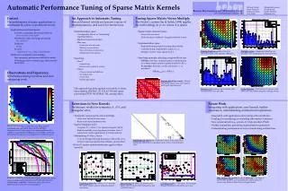
Explore the motivation and techniques for automatic performance tuning of sparse matrix kernels, maximizing software speed while simplifying programming. Learn about the BEBOP project and optimization results. Discover the impact of tuning dense BLAS, SpMV performance, and register tile sizes on various architectures.

E N D
Automatic Performance TuningSparse Matrix Kernels James Demmel www.cs.berkeley.edu/~demmel/cs267_Spr05
Berkeley Benchmarking and OPtimization (BeBOP) • Prof. Katherine Yelick • Rich Vuduc • Many results in this talk are from Vuduc’s PhD thesis, www.cs.berkeley.edu/~richie • Rajesh Nishtala, Mark Hoemmen, Hormozd Gahvari • Eun-Jim Im, many other earlier contributors • bebop.cs.berkeley.edu
Outline • Motivation for Automatic Performance Tuning • Recent results for sparse matrix kernels • OSKI = Optimized Sparse Kernel Interface • Future Work
Motivation for Automatic Performance Tuning • Writing high performance software is hard • Make programming easier while getting high speed • Ideal: program in your favorite high level language (Matlab, Python, PETSc…) and get a high fraction of peak performance • Reality: Best algorithm (and its implementation) can depend strongly on the problem, computer architecture, compiler,… • Best choice can depend on knowing a lot of applied mathematics and computer science • How much of this can we teach? • How much of this can we automate?
Examples of Automatic Performance Tuning (1) • Dense BLAS • Sequential • PHiPAC (UCB), then ATLAS (UTK) • Now in Matlab, many other releases • math-atlas.sourceforge.net/ • Fast Fourier Transform (FFT) & variations • Sequential and Parallel • FFTW (MIT) • Widely used • www.fftw.org • Digital Signal Processing • SPIRAL: www.spiral.net (CMU) • MPI Collectives (UCB, UTK) • More projects, conferences, government reports, …
Examples of Automatic Performance Tuning (2) • What do dense BLAS, FFTs, signal processing, MPI reductions have in common? • Can do the tuning off-line: once per architecture, algorithm • Can take as much time as necessary (hours, a week…) • At run-time, algorithm choice may depend only on few parameters • Matrix dimension, size of FFT, etc. • Can’t always do off-line tuning • Algorithm and implementation may strongly depend on data only known at run-time • Ex: Sparse matrix nonzero pattern determines both best data structure and implementation of Sparse-matrix-vector-multiplication (SpMV) • BEBOP project addresses this
Tuning Dense BLAS– ATLAS Extends applicability of PHIPAC; Incorporated in Matlab (with rest of LAPACK)
Tuning Register Tile Sizes (Dense Matrix Multiply) 333 MHz Sun Ultra 2i 2-D slice of 3-D space; implementations color-coded by performance in Mflop/s 16 registers, but 2-by-3 tile size fastest Needle in a haystack
SpMV with Compressed Sparse Row (CSR) Storage Matrix-vector multiply kernel: y(i) y(i) + A(i,j)*x(j) for each row i for k=ptr[i] to ptr[i+1] do y[i] = y[i] + val[k]*x[ind[k]] Matrix-vector multiply kernel: y(i) y(i) + A(i,j)*x(j) for each row i for k=ptr[i] to ptr[i+1] do y[i] = y[i] + val[k]*x[ind[k]]
Motivation for Automatic Performance Tuning of SpMV • Historical trends • Sparse matrix-vector multiply (SpMV): 10% of peak or less • 2x faster than CSR with “hand-tuning” • Tuning becoming more difficult over time • Performance depends on machine, kernel, matrix • Matrix known at run-time • Best data structure + implementation can be surprising • Our approach: empirical modeling and search • Up to 4x speedups and 31% of peak for SpMV • Many optimization techniques for SpMV • Several other kernels: triangular solve, ATA*x, Ak*x • Release OSKI Library, integrate into PETSc
Example: The Difficulty of Tuning • n = 21216 • nnz = 1.5 M • kernel: SpMV • Source: NASA structural analysis problem • 8x8 dense substructure
Taking advantage of block structure in SpMV • Bottleneck is time to get matrix from memory • Only 2 flops for each nonzero in matrix • Don’t store each nonzero with index, instead store each nonzero r-by-c block with index • Storage drops by up to 2x, if rc >> 1, all 32-bit quantities • Time to fetch matrix from memory decreases • Change both data structure and algorithm • Need to pick r and c • Need to change algorithm accordingly • In example, is r=c=8 best choice? • Minimizes storage, so looks like a good idea…
Best: 4x2 Reference Speedups on Itanium 2: The Need for Search Mflop/s Mflop/s
Register Profile: Itanium 2 1190 Mflop/s 190 Mflop/s
Ultra 2i - 9% 63 Mflop/s Ultra 3 - 5% 109 Mflop/s SpMV Performance (Matrix #2): Generation 2 35 Mflop/s 53 Mflop/s Pentium III - 19% Pentium III-M - 15% 96 Mflop/s 120 Mflop/s 42 Mflop/s 58 Mflop/s
Ultra 2i - 11% 72 Mflop/s Ultra 3 - 5% 90 Mflop/s Register Profiles: Sun and Intel x86 35 Mflop/s 50 Mflop/s Pentium III - 21% Pentium III-M - 15% 108 Mflop/s 122 Mflop/s 42 Mflop/s 58 Mflop/s
Power3 - 13% 195 Mflop/s Power4 - 14% 703 Mflop/s SpMV Performance (Matrix #2): Generation 1 100 Mflop/s 469 Mflop/s Itanium 1 - 7% Itanium 2 - 31% 225 Mflop/s 1.1 Gflop/s 103 Mflop/s 276 Mflop/s
Power3 - 17% 252 Mflop/s Power4 - 16% 820 Mflop/s Register Profiles: IBM and Intel IA-64 122 Mflop/s 459 Mflop/s Itanium 1 - 8% Itanium 2 - 33% 247 Mflop/s 1.2 Gflop/s 107 Mflop/s 190 Mflop/s
Example: The Difficulty of Tuning • n = 21216 • nnz = 1.5 M • kernel: SpMV • Source: NASA structural analysis problem
Zoom in to top corner • More complicated non-zero structure in general
3x3 blocks look natural, but… • More complicated non-zero structure in general • Example: 3x3 blocking • Logical grid of 3x3 cells • But would lead to lots of “fill-in”
Extra Work Can Improve Efficiency! • More complicated non-zero structure in general • Example: 3x3 blocking • Logical grid of 3x3 cells • Fill-in explicit zeros • Unroll 3x3 block multiplies • “Fill ratio” = 1.5 • On Pentium III: 1.5x speedup! • Actual mflop rate 1.52 = 2.25 higher
Automatic Register Block Size Selection • Selecting the r x c block size • Off-line benchmark • Precompute Mflops(r,c) using dense A for each r x c • Once per machine/architecture • Run-time “search” • Sample A to estimate Fill(r,c) for each r x c • Run-time heuristic model • Choose r, c to maximize Mflops(r,c) / Fill(r,c)
Accurate and Efficient Adaptive Fill Estimation • Idea: Sample matrix • Fraction of matrix to sample: sÎ [0,1] • Cost ~ O(s * nnz) • Control cost by controlling s • Search at run-time: the constant matters! • Control s automatically by computing statistical confidence intervals • Idea: Monitor variance • Cost of tuning • Lower bound: convert matrix in 5 to 40 unblocked SpMVs • Heuristic: 1 to 11 SpMVs
Accuracy of the Tuning Heuristics (1/4) See p. 375 of Vuduc’s thesis for matrices NOTE: “Fair” flops used (ops on explicit zeros not counted as “work”)
Evaluating algorithms and machines for SpMV • Metrics • Speedups • Mflop/s (“fair” flops) • Fraction of peak • Questions • Speedups are good, but what is “the best?” • Independent of instruction scheduling, selection • Can SpMV be further improved or not? • What machines are “good” for SpMV?
Upper Bounds on Performance for blocked SpMV • P = (flops) / (time) • Flops = 2 * nnz(A) • Lower bound on time: Two main assumptions • 1. Count memory ops only (streaming) • 2. Count only compulsory, capacity misses: ignore conflicts • Account for line sizes • Account for matrix size and nnz • Charge minimum access “latency” ai at Li cache & amem • e.g., Saavedra-Barrera and PMaC MAPS benchmarks
Example: L2 Misses on Itanium 2 Misses measured using PAPI [Browne ’00]
Achieved Performance and Machine Balance • Machine balance [Callahan ’88; McCalpin ’95] • Balance = Peak Flop Rate / Bandwidth (flops / double) • Lower is better (I.e. can hope to get higher fraction of peak flop rate) • Ideal balance for mat-vec: £ 2 flops / double • For SpMV, even less
Where Does the Time Go? • Most time assigned to memory • Caches “disappear” when line sizes are equal • Strictly increasing line sizes
Summary: Performance Upper Bounds • What is the best we can do for SpMV? • Limits to low-level tuning of blocked implementations • Refinements? • What machines are good for SpMV? • Partial answer: balance characterization • Architectural consequences? • Help to have strictly increasing line sizes
Summary of Other Performance Optimizations • Optimizations for SpMV • Register blocking (RB): up to 4x over CSR • Variable block splitting: 2.1x over CSR, 1.8x over RB • Diagonals: 2x over CSR • Reordering to create dense structure + splitting: 2x over CSR • Symmetry: 2.8x over CSR, 2.6x over RB • Cache blocking: 2.8x over CSR • Multiple vectors (SpMM): 7x over CSR • And combinations… • Sparse triangular solve • Hybrid sparse/dense data structure: 1.8x over CSR • Higher-level kernels • AAT*x, ATA*x: 4x over CSR, 1.8x over RB • A2*x: 2x over CSR, 1.5x over RB
Raefsky4 (structural problem) + SuperLU + colmmd N=19779, nnz=12.6 M Dense trailing triangle: dim=2268, 20% of total nz Can be as high as 90+%! 1.8x over CSR Example: Sparse Triangular Factor
“axpy” dot product Cache Optimizations for AAT*x • Cache-level: Interleave multiplication by A, AT … … • Register-level: aiT to be r´c block row, or diag row • Algorithmic-level transformations for A2*x, A3*x, …
Example: Combining Optimizations • Register blocking, symmetry, multiple (k) vectors • Three low-level tuning parameters: r, c, v X k v * r c += Y A