Download
1 / 50
500 likes | 534 Views
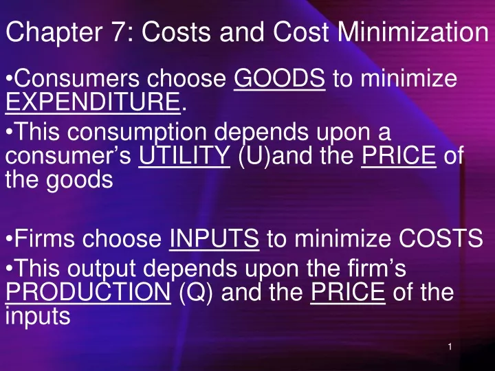
Chapter 7: Costs and Cost Minimization. Consumers choose GOODS to minimize EXPENDITURE . This consumption depends upon a consumer’s UTILITY (U)and the PRICE of the goods Firms choose INPUTS to minimize COSTS

E N D
Chapter 7: Costs and Cost Minimization • Consumers choose GOODS to minimize EXPENDITURE. • This consumption depends upon a consumer’s UTILITY (U)and the PRICE of the goods • Firms choose INPUTS to minimize COSTS • This output depends upon the firm’s PRODUCTION (Q) and the PRICE of the inputs
Chapter 7: Costs and Cost Minimization In this chapter we will cover: 7.2 Isocost Lines 7.3 Cost Minimization 7.4 Short-Run Cost Minimization
Cost Minimization • One of the goals of a firm is to produce output at a minimum cost. • This minimization goal can be carried out in two situations: • The long run (where all inputs are variable) • The short run (where some inputs are not variable)
The (Long Run) Cost Minimization Problem Suppose that a firm’s owners wish to minimize costs… Let the desired output be Q0 Technology: Q = f(L,K) Owner’s problem: min TC = rK + wL K,L Subject to Q0 = f(L,K)
7.2 The Isocost Line • From the firm’s cost equation: • TC0 = rK + wL • One can obtain the formula for the ISOCOST LINE: • K = TC0/r – (w/r)L • The isocost line graphically depicts all combinations of inputs (labour and capital) that carry the same cost.
K Example: Isocost Lines Direction of increase in total cost TC2/r TC1/r Slope = -w/r TC0/r L TC0/w TC1/w TC2/w
7.3 Cost Minimization Isocost curves are similar to budget lines, and the tangency condition of firms is also similar to the tangency condition of consumers: MRTSL,K = -MPL/MPK = -w/r
K Example: Cost Minimization TC2/r • Cost inefficient point for Q0 TC1/r Cost minimization point for Q0 TC0/r • Isoquant Q = Q0 L TC0/w TC1/w TC2/w
Cost Minimization Steps • Tangency Condition • - MPL/MPK = w/r-gives relationship between L and K • 2) Substitute into Production Function • -solves for L and K • 3) Calculate Total Cost • 4) Conclude
Example: Interior Solution • Q = 50L1/2K1/2 w = $5 r = $20 • MPL = 25K1/2/L1/2 Q0 = 1000 • MPK = 25L1/2/K1/2 1) Tangency:MPL/MPK = w/r (25K1/2/L1/2)/(25L1/2/K1/2)=w/rK/L = 5/20 L=4K
Example: Interior Solution 2) Substitution: 1000 = 50L1/2K1/2 1000 = 50(4K)1/2K1/2 1000=100K K = 10 L = 4K L = 4(10)L = 40
Example: Interior Solution 3) Total Cost: TC0 = rK + wL TC0 = 20(10) + 5(40) TC0 = 400 4) Conclude Cost is minimized at $400 when labour is 40 and capital is 10.
K Example: Interior Solution 400/r Cost minimization point • 10 Isoquant Q = 1000 L 40 400/w
Example: Corner Solution • Q = 10L + 2K • MPL = 10 • MPK = 2 • w = $5 • r = $2 • Q0 = 200 1) Tangency Condition:MPL/MPK = w/r 10/2=5/2 10=5???? Tangency condition fails!
Example: Corner Solution • We can rewrite the tangency condition: • MPL/w = MPK /r • -the productivity per dollar for labour is equal to the productivity per dollar for capital • -but here: • MPL/w = 10/5 > MPK /r = 2/2 • …the “bang for the buck” in labour is ALWAYS larger than the “bang for the buck” in capital… • So you would only use labor:
Example: Corner Solution • 2) Substitution (K=0) • Q = 10L + 2K200 = 10L + 2(0) • = L • 3) Total Cost • TC0 = rK + wL • TC0 = 2(0) + 5(20) • TC0 = 100 4) Conclude Cost is minimized at $100 when labour is 20 and capital is zero.
Example: Cost Minimization: Corner Solution K Isoquant Q = Q0 • L Cost-minimizing input combination
Comparative Statistics • The isocost line depends upon input prices and desired output • Any change in input prices or output will shift the isocost line • This shift will cause changes in the optimal choice of inputs
Comparative Statics • A change in the relative price of inputs changes the slope of the isocost line. If MRTSL,K is decreasing, An increase in wage:-decreases the cost minimizing quantity of labour -increases the cost minimizing quantity of capital An increase in rent -decreases the cost minimizing quantity of capital -increases the cost minimizing quantity of labour.
Example: Change in Relative Prices of Inputs K Cost minimizing input combination w=2, r=1 • Cost minimizing input combination, w=1, r=1 Isoquant Q = Q0 • 0 L
Example • Originally, MicroCorp faced input prices of $10 for both labor and capital. MicroCorp has a contract with its parent company, Econosoft, to produce 100 units a day through the production function: • Q=2(LK)1/2 • MPL=(K/L)1/2 MPK=(L/K)1/2 • If the price of labour increased to $40, calculate the effect on capital and labour.
Example • If the price of labour quadruples from $10 to $40… • Labour will be cut in half, from 50 to 25 • Capital will double, from 50 to 100
Comparative Statics • An increase in Q0 moves the isoquant Northeast. • The cost minimizing input combinations, as Q0 varies, trace out the expansion path • If the cost minimizing quantities of labor and capital rise as output rises, labor and capital are normal inputs • If the cost minimizing quantity of an input decreases as the firm produces more output, the input is called an inferior input
K Example: An Expansion Path TC2/r TC1/r Expansion path, normal inputs • TC0/r • Isoquant Q = Q0 • L TC0/w TC1/w TC2/w
K Example: An Expansion Path TC2/r Expansion path, labour is inferior • TC1/r • L TC1/w TC2/w
Example • Originally, MicroCorp faced input prices of $10 for both labor and capital. MicroCorp has a contract with its parent company, Econosoft, to produce 100 units a day through the production function: • Q=2(LK)1/2 • MPL=(K/L)1/2 MPK=(L/K)1/2 • If Econosoft demanded 200 units, how would labour and capital change?
Example • If the output required doubled from 100 to 200.. • Labour will double, from 50 to 100 • Capital will double, from 50 to 100 (Constant Returns to Scale)
Input Demand Functions • The demand curve for INPUTS is a schedule of amount of input demanded at each given price level (Also known as FACTOR DEMAND) • This demand curve is derived from each individual firm minimizing costs: Definition: The cost minimizing quantities of labor and capital for various levels of Q, w and r are the input demand functions. L = L*(Q,w,r) K = K*(Q,w,r)
K Example: Labour Demand Function • • When input prices (wage and rent, etc) change, the firm maximizes using different combinations of inputs. • Q = Q0 W3/r W2/r W1/r 0 L w As the price of inputs goes up, the firm uses LESS of that input, as seen in the input demand curve • • • L*(Q0,w,r) L1 L2 L3 L
K • • A change in the quantity produced will shift the isoquant curve. • • Q = Q0 • • Q = Q1 0 L w This will result in a shift in the input demand curve. • • • • • L*(Q0,w,r) • L*(Q1,w,r) L1 L2 L3 L
Calculating Input demand functions • Use the tangency condition to find the relationship between inputs: • MPL/MPK = w/rK=f(L) or L=f(K) • 2) Substitute above into production function and solve for other variable: • Q=f(L,K), K=f(L) =>L=f(Q) • Q=f(L,K), L=f(K) =>K=f(Q)
Example: Input demand functions • Q = 50L1/2K1/2 • MPL=25(K/L)1/2, MPK=25(L/K)1/2 • Tangency Condition: • MPL/MPK = w/r • K/L = w/r • K=(w/r)L • or • L=(r/w)K
Example: Input demand functions 2) Production Function Q0 = 50L1/2K1/2 Q0 = 50L1/2[(w/r)L]1/2 L*= (Q0/50)(r/w)1/2 or Q0 = 50 [(r/w)K]1/2K1/2 K*= (Q0/50)(w/r)1/2 • Labor and capital are both normal inputs • Labor is a decreasing function of w • Labor is an increasing function of r
Price Elasticity of Demand (Inputs) • Price elasticity of demand can be calculated for inputs (Factor markets) similar to outputs:
Example • JonTech produces the not-so-popular J-Pod. • JonTech faces the following situation: • Q*=5(KL)1/2=100 • MRTS=K/L. • w=$20 and r=$20 • Calculate the Elasticity of Demand for Labour if wages drop to $5.
Example • Initially: • MRTS=K/L=w/r • K=20L/20 • K=L • Q=5(KL)1/2 • 100=5K • 20=K=L
Example • After Wage Change: • MRTS=K/L=w/r • K=5L/20 • 4K=L • Q=5(KL)1/2 • 100=10K • 10=K • 40=L
Example • Price Elasticity of Labour Demand:
7.4 Short Run Cost Minimization Cost minimization occurs in the short run when one input (generally capital) is fixed (K*). Total variable cost is the amount spent on the variable input(s) (ie: wL) -this cost is nonsunk (can be avoided) Total fixed cost is the amount spent on fixed inputs (ie: rK*) -if this cost cannot be avoided, it is sunk -if this cost can be avoided, it is nonsunk (ie: rent factory to another firm)
Short Run Cost Minimization Cost minimization in the short run is easy: Min TC=wL+rK* L s.t. the constraint Q=f(L,K*) Where K* is fixed.
Short Run Cost Minimization Example: Minimize the cost to build 80 units if Q=2(KL)1/2 and K=25. Q=2(KL)1/2 80=2(25L)1/2 80=10(L)1/2 8=(L)1/2 64=L Notice that price doesn’t matter.
K Short Run Cost Minimization TC2/r TC1/r Long-Run Cost Minimization • Short-Run Cost Minimization • K* L TC1/w TC2/w
Short Run Expansion Path Choosing 1 input in the short run doesn’t depend on prices, but it does depend on quantity produced. The short run expansion path shows the increased demand for labour as quantity produced increases: (next slide) The demand for inputs will therefore vary according to quantity produced. (The demand curve for inputs shifts when production changes)
K Example: Short and Long Run Expansion Paths TC2/r Long Run Expansion Path TC1/r • TC0/r • • • Short Run Expansion Path K* • L TC0/w TC1/w TC2/w
Short Run and Many Inputs If the Short-Run Minimization problem has 1 fixed input and 2 or more variable inputs, it is handled similarly to the long run situation:
Chapter 7 Key Concepts • The Isocost line gives all combinations of inputs that have the same cost • Costs are minimized when the Isocost line is tangent to the Isoquant • When input costs change, the minimization point (and minimum cost) changes • When required output changes, the minimization point (and minimum cost) changes • The creates the expansion path
Chapter 7 Key Concepts • Individual firm choice drives input demand • As input prices change, input demanded changes • There are price elasticities of inputs • In the short run, at least one factor is fixed • Short run expansion paths differ from long run expansion paths