Download
1 / 17
170 likes | 175 Views
Beamdiagnostics by Beamstrahlung Pair Analysis. C.Grah – DESY FCAL Collaboration Workshop MPI Munich, 17 th October 2006. Content. Overview Geometries and Parameter Sets Beamstrahlung Pair Analysis Results of Pair Analysis

E N D
Beamdiagnostics by Beamstrahlung Pair Analysis C.Grah – DESY FCAL Collaboration Workshop MPI Munich, 17th October 2006
Content • Overview • Geometries and Parameter Sets • Beamstrahlung Pair Analysis • Results of Pair Analysis • Comparison between 2mrad, and 14mrad for different magnetic field configurations • Look on the Geant4 Simulation BeCaS and first results (A.Sapronov) C.Grah: Beamdiagnostics
The New Baseline – 14mrad 14mrad • The reduce overall costs (two different interaction regions) the new baseline is: • two IR‘s with 14mrad crossing angle • We should be prepared for both magnetic field configurations: DID and Anti-DID • Choose to keep the same geometry as for 20mrad until now. • For 20mrad we should increase the aperture of LumiCal even more (~120mm). Origin of backscattered particles for 20mrad Ant-iDID. (A.Vogel) 100 BX C.Grah: Beamdiagnostics
Under Discussion – LowP Parameter Set • A further significant cost descrease of the ILC could be achieved by: ½ RF power • IF we want to achieve the same luminosity the beam parameters will be quite aggressive • Nbunch = 2880 => 1330 • εy = 40 => 35 x 10-9m rad • σx = 655 => 452 nm • σy = 5.7 => 3.8 nm • σz = 300 => 200 μm • δBS = 2.2 => 5.7 % Energy from pairs in BeamCal per BX C.Grah: Beamdiagnostics
Pair Distributions for 14mrad Nominal LowP DID Anti DID Larger blind area compared to 20 mrad (30° => 40°) C.Grah: Beamdiagnostics
Beamstrahlung Pair Analysis e- e+ Interaction γ e- e- Creation of beamstrahlung (Nphot~ O(1) per bunch particle δBS~ O(1%) energy loss) Production of incoherent e+e- pairs • e+e- pairs from beamstrahlung are deflected into the BeamCal • 15000 e+e- per BX => 10 – 20 TeV • ~ 10 MGy per year => radiation hard sensors • The spectra and spatial distribution contain information about the initial collision. C.Grah: Beamdiagnostics
Fast Luminosity Monitoring Simulation of the Fast Feedback System of the ILC. Development of the Luminosity during the first 600 bunches of a train. Ltotal = L(1-600) + L(550-600)*(2820-600)/50 position and angle scan G.White QMUL/SLAC RHUL & Snowmass presentation • Standard procedur (using BPMs) • Include pair signal (N) as additional input to the sytsem • Increase of luminosity of 10 - 15% C.Grah: Beamdiagnostics
Concept of the Beamstrahlung Pair Analysis Simulate Collision with Guineapig 1.) nominal parameter set 2.) with variation of a specific beam parameter (e.g. σx, σy, σz, Δσx, Δσy, Δσz) Produce photon/pair output ASCII File A.Sapronov: BeCaS1.0 A.Stahl: beammon.f Extrapolate pairs to BeamCal front face and determine energy deposition (geometry and magnetic field dependent) Run full GEANT4 simulation BeCaS and calculate energy deposition per cell (geometry and magnetic field dependent) Calculate Observables and write summary file Calculate Observables and write summary file Do the parameter reconstruction using 1.) linear approximation (Moore Penrose Inversion Method) 2.) using fits to describe non linear dependencies LC-DET-2005-003 Diagnostics of Colliding Bunches from Pair Production and Beam Strahlung at the IP Achim Stahl C.Grah: Beamdiagnostics
Moore Penrose Method Taylor Matrix ΔBeamPar Observables Observables = + * nom • Observables (examples): • total energy • first radial moment • thrust value • angular spread • E(ring ≥ 4) / Etot • E / N • l/r, u/d, f/b asymmetries detector: realistic segmentation, ideal resolution, bunch by bunch resolution C.Grah: Beamdiagnostics
1st order Taylor Matrix parametrization (polynomial) 1 point = 1 bunch crossing by guinea-pig slope at nom. value taylor coefficient i,j observable j [au] beam parameter i [au] C.Grah: Beamdiagnostics
Beam Parameter Reconstruction Single parameter reconstruction C.Grah: Beamdiagnostics
Beam Parameter Reconstruction Beamparameters vs Observables slopes (significance) normalized to sigmas 2mrad 14mrad DID C.Grah: Beamdiagnostics
Tauchi Observables • Tauchi & Yokoya, Phys Rev E51, (1995) 6119 Define 2 x 2 regions with: high energy deposition low energy deposition Tauchi1 = (Low1 + Low2)/(High1+High2) Tauchi2= High1/High2 Has to be redefined for each geometry/ magnetic field. Optimum not found yet. C.Grah: Beamdiagnostics
Geant 4 Simulation - BeCaS 2mrad • A Geant4 BeamCal simulation has been set up by A.Sapronov. • Energy distribution for 2mrad and 20mrad DID (14mrad not yet simulated). • BeCaS can be configured to run with: • different crossing angles (according geometry is chosen) • magnetic field (solenoid, (Anti) DID, use field map • detailed material composition of BeamCal including sensors with metallization, absorber, PCB, air gap 20mrad C.Grah: Beamdiagnostics
BeCaS - Checkplots C.Grah: Beamdiagnostics
Beamparameter Reconstruction • Using the observables: • Etot // (1) Total energy • Rmom // (2) Average radius • Irmom // (3) radial moment • UDimb // (4) U-D imbalance • RLimb // (5) R-L imbalance • Eout // (6) Energy with r>=6 • PhiMom // (7) Phi moment • NoverE // (15) N/E C.Grah: Beamdiagnostics
Summary • The geometry for a 14mrad beam crossing angle is the same as for 20mrad. The 20mrad geometry should be changed due to background. • The LowP parameter set is under discussion => lower L or higher background. • Consolidated guineapig steering parameters and reproduced pair/photon files. • Tested 2, 14 and 20 mrad configurations with DID/AntiDID field. • Found small significance of the Tauchi variables. • A Geant4 simulation of BeamCal (BeCaS) is ready for usage. First tests show that a subset of the detector information seems sufficient for beam parameter reconstruction. • Include this into Mokka • Build additional fast FCAL simulation (?) C.Grah: Beamdiagnostics