Download
1 / 68
680 likes | 689 Views
This study explores the source waters, flowpaths, and solute flux in mountain catchments, focusing on snowmelt and the challenges posed by fractured rock environments. The research site is Green Lake Valley, where various water samples were collected and analyzed. Mixing models and isotopic fractionation were used to understand the flow of water and tracers. End-member mixing analysis (EMMA) and matrix operations were employed to quantitatively evaluate the results.

E N D
Source waters, flowpaths, and solute flux in mountain catchments Mark Williams
SNOWMELT Mountain-Block Recharge (MBR) + Stream Infiltration Mountain-Front Recharge (MFR)
HYDROLOGIC UNKNOWNS • Flowpaths • Residence time • Circulation depth • Reservoir sizes • Groundwater fluxes • Fractured rock environment increases difficulty of understanding mountain plumbing Add snowmelt runoff Permafrost
APPLICATION IN GREEN LAKES VALLEY: LTER RESEARCH SITE Green Lake 4 • Sample Collection • Stream water - weekly grab samples • Snowmelt - snow lysimeter • Soil water - zero tension lysimeter • Talus water – biweekly to monthly • Sample Analysis • Delta 18O and major solutes
MIXING MODEL: 2 COMPONENTS • One Conservative Tracer • Mass Balance Equations for Water and Tracer
ASSUMPTIONS FOR MIXING MODEL • Tracers are conservative (no chemical reactions); • All components have significantly different concentrations for at least one tracer; • Tracer concentrations in all components are temporally constant or their variations are known; • Tracer concentrations in all components are spatially constant or treated as different components; • Unmeasured components have same tracer concentrations or don’t contribute significantly.
d18O IN SNOW AND STREAMFLOW • d18O fractionation of 4%o in snowmelt; • Cannot use d18O values measured at snow lysimeter directly to the catchment. • Failed assumption
Fractionation in Snowpack d18O = -20‰ Snow surface Ground Difference between maximum 18O values and Minimum 18O values about 4 ‰ d18O = -22‰
Isotopic Fractionation • Fractionation occurs as melt from surface percolates towards bottom of snowpack • Isotopic exchange between ice and percolating liquid water • d18Osolid > d18Oliquid > d18Ovapour • Molecules of surface meltwater are not the same as the ones at the base of the snowpack
ACCOUNTING FOR d18O IN MELTWATER • d18O values are highly correlated with amount of melt (R2 = 0.9, n = 15, p < 0.001); • Snowmelt regime is different at a point from a real catchment; • So, we developed a Monte Carlo procedure to stretch the dates of d18O in snowmelt measured at a point to a catchment scale using the streamflow d18O values.
NEW WATER FROM VARIOUS MODELS M1 - Original time-series of snowpack d18O M2 - Date-stretched time-series of snowpack d18O M3 - Original time-series of snowmelt lysimeter d18O M4 - Date-stretched time-series of snowmelt lysimeter d18O
NEW WATER AND OLD WATER Old Water = 64% Not Teflon basins!
MIXING MODEL: 3 COMPONENTS Simultaneous Equations Solutions • Two Conservative Tracers • Mass Balance Equations for Water and Tracers Q - Discharge C - Tracer Concentration Subscripts - # Components Superscripts - # Tracers
MIXING MODEL: 3 COMPONENTS(Using Discharge Fractions) Simultaneous Equations Solutions • Two Conservative Tracers • Mass Balance Equations for Water and Tracers f - Discharge Fraction C - Tracer Concentration Subscripts - # Components Superscripts - # Tracers
FLOWPATHS: 2-TRACER 3-COMPONENT MIXING • Did we choose the right end-members? • Did we choose the right tracers? • Is there any way to quantitatively • evaluate our results?
END-MEMBER MIXING ANALYSIS (EMMA) • Uses more tracers than components • Decides number of end-members • Quantitatively select end-members • Quantitatively evaluate results of the • mixing model
MIXING MODEL: Generalization Using Matrices Simultaneous Equations Where • One tracer for 2 components and two tracers for 3 components • N tracers for N+1 components? -- Yes • However, solutions would be too difficult for more than 3 components • So, matrix operation is necessary Solutions • Note: • Cx-1 is the inverse matrix of Cx • This procedure can be generalized to N tracers for N+1 components
EMMA PROCEDURES • Identification of Conservative Tracers - Bivariate solute-solute plots to screen data; • PCA Performance - Derive eigenvalues and eigenvectors; • Orthogonal Projection - Use eigenvectors to project chemistry of streamflow and end-members; • Screen End-Members - Calculate Euclidean distance of end-members between their original values and S-space projections; • Hydrograph Separation - Use orthogonal projections and generalized equations for mixing model to get solutions! • Validation of Mixing Model - Predict streamflow chemistry using results of hydrograph separation and original end-member concentrations.
STEP 1 - MIXING DIAGRAMS • Look familiar? • This is the same diagram used for geometrical definition of mixing model (components changed to end-members); • Generate all plots for all pair-wise combinations of tracers; • The simple rule to identify conservative tracers is to see if streamflow samples can be bound by a polygon formed by potential end-members or scatter around a line defined by two end-members; • Be aware of outliers and curvature which may indicate chemical reactions!
STEP 2 - PCA PERFORMANCE • For most cases, if not all, we should use correlation matrix rather than covariance matrix of conservative solutes in streamflow to derive eigenvalues and eigenvectors; • Why? This treats each variable equally important and unitless; • How? Standardize the original data set using a routine software or minus mean and then divided by standard deviation; • To make sure if you are doing right, the mean should be zero and variance should be 1 after standardized!
APPLICATION OF EIGENVALUES • Eigenvalues can be used to infer the number of end-members that should be used in EMMA. How? • Sum up all eigenvalues; • Calculate percentage of each eigenvalue in the total eigenvalue; • The percentage should decrease from PCA component 1 to p (remember p is the number of solutes used in PCA); • How many eigenvalues can be added up to 90% (somewhat subjective! No objective criteria for this!)? Let this number be m, which means the number of PCA components should be retained (sometimes called # of mixing spaces); • (m +1) is equal to # of end-members we use in EMMA.
PCA PROJECTIONS First 2 eigenvalues are 92% and so 3 end-members appear to be correct!
NIWOT RIDGE NADP SITE: N-DEP INCREASED > 4x
Potential Sources of Nitrate and Ammonium
EMMA: NITRATE SOURCES • Under-predicts nitrate during snowmelt • Ionic pulse important • Overpredicts nitrate during summer • Denitrification? • 8-ha Martinelli: 30% stream nitrate atmos • 225-ha GL4: 20% stream nitrate atmos
Dual isotopic • analysis of • nitrate • d18O (no3) • d15N (no3)
DUAL ISOTOPE: NITRATE SOURCES • 8-ha Martinelli: 60% stream nitrate atmos • Twice EMMA • 225-ha GL4: 20% stream nitrate atmos • Same as EMMA
EMMA and NITRATE ISOTOPES • First time used together • 20% atmospheric nitrate in 220-ha stream • EMMA, dual isotopes similar results • 60% atmospheric nitrate in 8-ha stream • EMMA underestimates: unsampled flowpath • Talus nitrate microbial, not atmospheric • Denitrification probably very important
1 1,300 river miles in Colordo 100,000 AMD sites in Western US
END OF PIPE TREATMENT STRATEGY • Millions of dollars to install • Expensive to operate • Operate for long-term • Need low-cost alternatives
Watershed approach, hydrometric, isotopic, and chemical measurements CHALK CREEK MINE:GROUNDWATER SOURCE CONTROLSDEMONSTRATION PROJECT EPA VIII 104(b)3 Program SUPPLEMENTAL FUNDING REQUEST Assistance Agreement MM998404-02