State Feedback for Discrete-Time Systems

1. State Feedback for Discrete-Time Systems Pole Placement, State Estimation, Integral Control, LQR, Kalman Estimators M.V. Iordache, EEGR4933 Automatic Control Systems, Spring 2019, LeTourneau University

2. Input Input Output Output r(t) r(t) y(t) y(t) State Space Representation • Discrete time representation • Recall the continuous time representation

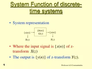
3. Input Output r(t) y(t) Input Output r(t) y(t) Relation between SS and TF models • Conversions TF  SS and SS  TF possible.

4. Input Output r(t) y(t) Transfer Function of SS Model • Assumes zero initial conditions: x(0) = 0.

5. Input Output r(t) y(t) Solution of the SS equation • Note that y(k) and x(k) depend on • x(0) – the initial state • r(k) – the input

6. Stability • BIBO stability: necessary for most engineering systems. • For SS models: x(k) is also required to be bounded. • For stability, all eigenvalues of A must be inside the unit circle. • This ensures more than just boundedness: • If r(k)  rSS then x(k)  xSS = – (A – I)-1BrSS • In particular, for zero input, x(k) decays exponentially from x(0) to 0.

7. Controllability • Is there for any x(0) some input u(k) that leads in finite time the state x to the origin? If yes, the system is (completely state) controllable (controllable to the origin). • Is there for any state s some input u(k) that leads in finite time the state x from the origin to s? If yes, the system is reachable (controllable from the origin). • Reachability implies that for any k1, z1, and z2, there is k2>k1 and some input u(k) that transfers the state from x(k1) = z1 to x(k2) = z2.

8. Controllability • Reachability implies controllability. • If A is invertible, controllability implies reachability. • Assume n state variables. • The system is reachable when the controllability matrix has rank n (full rank).

9. Observability • Is there some finite time k1 such that x(0) can be determined from u(0), u(1), …, u(k1) and y(0), y(1), …, y(k1)? If yes, the system is (completely state) observable. • The system is observable when the observability matrix has rank n (full rank).

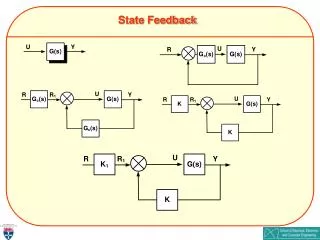
10. State Feedback • In output feedback, the input depends on the output. • In state feedback, the input depends on the state. • Linear state feedback • State feedback changes the position of the eigenvalues λ of the system. Now they satisfy:

11. State Feedback • K determines the poles of the system. • Arbitrary pole placement is possible for systems that are reachable (controllable from the origin). • Pole placement can be used to: • Stabilize an unstable system by placing all poles inside the unit circle. • Make a stable system faster by moving the dominant pole(s) away from the unit circle.

12. Ackerman’s Formula • Let λ1, λ2, …, λn, be the desired eigenvalues. • Let • For single-input reachable systems, the following gain achieves the desired poles: • IMPORTANT: if A is , then must have the order .

13. Where to Place the Poles • Let be the sampling interval. • If is a desired pole in the s-domain, use in the z-domain. • Normally, the poles will be very close to the unit circle. • The dominant pole is the pole closest to the unit circle. • Single dominant pole 1st order response • Pair of complex conjugate dominant poles  2nd order response. • An approximate formula relating the dominant pole to the 2% settling time to a step input is: where • The approximation is good if . • To find as a discrete time, use .

14. Pole Placement Limitations • Linear models are usually valid for small enough inputs. • Actuators may not be able to apply the requested input if the desired response is too fast. • Typically the state x cannot be measured directly  state estimation.

15. State Estimation • Typically the state x cannot be measured directly. However, we can estimate it based on the plant model, y, and u. • Correction term needed because • x(0) is unknown. • Models are not precise. • There are disturbances and measurement noise.

16. State Estimation • Ideally, the estimation error converges to zero if the eigenvalues of are inside the unit circle. • If is stable, the error converges to zero even if . However, a nonzero can make converge faster to 0. • will not converge to zero if the effect of measurement noise, disturbances, and modeling error is accounted for.

17. Closed-Loop with State Estimation • The input of the plant is • Here, the estimate is used for instead of , which is unavailable. • The estimator gain and the feedback gain can be designed independently. • However, the estimator should be faster than the closed-loop system. Example: If is a dominant CL pole, the dominant estimator pole could be chosen so that .

18. Closed-Loop with State Estimation The textbook states that: • A rule of thumb often stated is to make the estimator two to four times faster than the system. • So . • State estimation can be dangerous, since the plant is controlled based on estimates and not actual state measurements. • … great care must be exercised to ensure that the effects of the estimator are well understood for all possible conditions of system operation.

19. Deadbeat Control • Steady state reached in a finite (and small) number of steps. Deadbeat response Non-deadbeat response

20. Deadbeat Control • Corresponds to FIR closed-loop transfer functions. • If n is the order of the FIR and a unit step input is applied, the output reaches its steady state after n sampling periods. • In sampled data systems, deadbeat control is practical for low sampling rates. • Design: Given A, B, C, D, place all poles at zero. • The ideal state estimator has the same matrices A, B, C, D, and so does not change the transfer function.

21. Integral Control • Approach: • Define new state variable(s): • Design stabilizing state feedback controller. • How it works: assume that the inputs converge to a constant steady state. Then:

22. Integral Control • Note the ss representation: • Proportional + integral terms:

23. LQR Design • Provides a different way to find K. • Pole placement finds K such that the poles are at the desired location. • LQR finds K that minimizes a cost function. • Suppose that should converge to zero. The LQR cost function is: • and select the terms that should converge faster to 0.

24. LQR Design • LQR finds that minimizes the cost function • The LQR solution has the form . • The solution is instead if • Note that .

25. Finite Horizon LQR • To find K, substitute and rewrite as • for , where:

26. LQR Design—Choosing Q & R • Suppose that • Select and . • Assign the largest weights to the most important goals. • Larger (compared to )  converges faster to 0. • Larger (compared to )  less power and energy required from actuator.

27. LQR Design—Choosing Q & R • Suppose that • Substitute and write in the form • Ensure and .

28. The Kalman Estimator • Real systems are affected by noise (v) and disturbances (w): • Since v and w are unknown, estimators always have some error. • The Kalman estimator minimizes the error.

29. The Kalman Estimator • The pole placement method: • Finds G that places poles at desired location. • Estimation error converges to zero assuming zero noise and disturbances. • The Kalman estimator method: • Finds G that minimizes estimation error. • The error is still zero for zero noise and disturbances. • The Kalman estimator is optimal under conditions that can be achieved only approximately in practice.

30. The Kalman Estimator • v and w are stochastic processes such that: • and . • , , and . • The Kalman estimator minimizes • Given Q, R, and N, G is calculated. The estimator has the same form:

31. The Kalman Estimator • Note that the estimate depends on output measurements up to time . • This can be stated explicitly by denoting as . • Note that the estimate depends on , that is, . • So depends on output measurements up to time . • Let denote .

32. The Kalman Estimator • So is an estimate of based on measurements up to time . • The innovation gain can be used to improve the estimate of when the measurement becomes available:

33. The Kalman Estimator • The function may be used in MATLAB. • It returns G, M, and an estimator object. • The estimator object (depending on options) outputs either • and . • or and .

34. LQG Design • Use the Kalman estimator for the state estimate. • Use the LQR design for the state feedback gain. • If TF of plant is given, convert TF to a state space model. • LQG and integral control can be combined.