Signal- und Bildverarbeitung, 323.014 Image Analysis and Processing Arjan Kuijper 16.11.2006

1. Signal- und Bildverarbeitung, 323.014Image Analysis and ProcessingArjan Kuijper16.11.2006 Johann Radon Institute for Computational and Applied Mathematics (RICAM) Austrian Academy of Sciences Altenbergerstraße 56A-4040 Linz, Austria arjan.kuijper@oeaw.ac.at

2. Summary of the previous weeks • Invariant differential feature detectors are special (mostly) polynomial combinations of image derivatives, which exhibit invariance under some chosen group of transformations. • The derivatives are easily calculated from the image through the multi-scale Gaussian derivative kernels. • The notion of invariance is crucial for geometric relevance. • Non-invariant properties have no value in general feature detection tasks. • A convenient paradigm to calculate features invariant under Euclidean coordinate transformations is the notion of gauge coordinates (v,w). • Any combination of derivatives with respect to v and w is invariant under Euclidean tranformations.

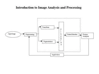
3. Today • The differential structure of images • Third order image structure: T-junction detection • Fourth order image structure: junction detection • Scale invariance and natural coordinates • Irreducible invariants • Geometry-driven diffusion • Adaptive smoothing and image evolution • Nonlinear diffusion equations • The Perona & Malik Equation • Scale-space implementation of the P&M equation • The P&M equation is ill-posed Taken from B. M. ter Haar Romeny, Front-End Vision and Multi-scale Image Analysis, Dordrecht, Kluwer Academic Publishers, 2003.Chapter 6/21

4. Gauge coordinates @ @ @ @ L L L L L L L ¡ + L L L ¡ ( ( ) ) ( ( ) ) @ @ @ @ Á Á Á Á Á Á r r r r i i i y x x x y x y y y y y ¡ x x x ¢ ¢ ¢ ¢ s c o n s s c o n s s c n o s = = = = = = = = v w v w p p p p p p p p ; ; ; ; 2 2 2 2 2 2 2 2 2 2 2 2 2 2 2 2 L L L L L L L L L L L L L L L L + + + + + + + + x x x x y y y y x x y y x x y y • Remind: • Do the trick: • And thus

5. Third order image structure: T-junction detection • T-junctions in the intensity landscape of natural images occur typically at occlusion points. Occlusion points are those points where a contour ends or emerges because there is another object in front of the contour.

6. Third order image structure: T-junction detection • When we zoom in on the T-junction of an observed image and inspect locally the isophote structure at a T-junction, we see that at a T-junction the derivative of the isophote curvature k in the direction perpendicular to the isophotes is high.

7. Third order image structure: T-junction detection 2 L L L L 2 ¡ + + v v w v v w w v w ¢ ¢ ¢ = 2 2 L L L w w w • When we study the curvature of the isophotes in the middle of the image, at the location of the T-junction, we see the isophote 'sweep' from highly curved to almost straight for decreasing intensity. • So the geometric reasoning is the "the isophote curvature changes a lot when we traverse the image in the w direction". • It seems to make sense to study

8. Third order image structure: T-junction detection • To avoid singularities at vanishing gradients through the division by we use as our T-junction detector:

9. Fourth order image structure: junction detection • Yet another order higher: Find in a checkerboard the crossings where 4 edges meet. • When we study the fourth order local image structure, we consider the fourth order polynomial terms from the local Taylor expansion. • The main theorem of algebra states that a polynomial is fully described by its roots. • How well all roots coincide, given by the discriminant, is a particular invariant condition. • The discriminant of second order image structure is just the determinant of the Hessian matrix, i.e. the Gaussian curvature.

10. Fourth order image structure: junction detection • The forth order discriminant is slightly more complicated:

11. Scale invariance and natural coordinates • The dimensionless coordinate is termed the natural coordinate. This implies that the derivative operator in natural coordinates has a scalingfactor: • Compare Lw and the natural Lw:

12. Irreducible invariants • It has been shown by Hilbert that any invariant of finite order can be expressed as a polynomial function of a set of irreducible invariants. For e.g. scalar images these invariants form the fundamental set of image primitives in which all local intrinsic properties can be described. • There are only a small number of irreducible invariants for low order. • E.g. for 2D images up to second order there are only 5 of such irreducibles. • One mechanism to find the irreducible set are gauge coordinates:

13. Tensors • There are many ways to set up an irreduciblebasis. • In tensor notation, tensor indices denote partial derivatives and run over the dimensionsso = and = • When indices come in pairs, summation over the dimensions is implied (the so-called Einstein summation convention, or contraction)

14. Tensors • Each of these irreducible invariants cannot be expressed in the others. Any invariant property to some finite order can be expressed as a combination of these irreducibles. Isophote curvature, a second order local invariant feature, is expressed as • These irreducibles form a basis for the differential invariant structure. The set of 5 irreducible grayvalue invariants in 2D images has been exploited to classify local image structure for statistical object recognition.

15. Geometry-driven diffusion

16. Adaptive Smoothing and Image Evolution • Calculate edges and other differential invariants at a range of scales. • Select a fine or a coarse scale? • Larger scale: • improved reduction of noise, • the appearance of more prominent structure, • localization accuracy. • Linear, isotropic diffusion cannot preserve the position of the differential invariant features over scale. • Make the diffusion (blurring) locally adaptive to the structure of the image. • preserve edges • reducing the noise

17. Adaptive Smoothing and Image Evolution • This adaptive filtering process is possible by three classes of (all nonlinear) mathematical approaches, which are in essence equivalent: • Nonlinear partial differential equations (PDE's), i.e. nonlinear diffusion equations which evolve the luminance function as some function of a flow. This general approach is known as the 'nonlinear PDE approach'; • Curve evolution of the isophotes (curves in 2D, surfaces in 3D) in the image. This is known as the 'curve evolution approach'. • Variational methods that minimize some energy functional on the image. This is known as the 'energy minimization approach' or 'variational approach'.

18. geometric reasoning • The word 'nonlinear' implies the inclusion of a nonlinearity in the algorithm. • This can be done in an infinite variety, and it takes geometric reasoning to come up with the right nonlinearity for the task. • We can include knowledge about • a preferred direction of diffusion, • or that we like the diffusion to be reduced at edges • or at points of high curvature • etc.

19. Nonlinear Diffusion Equations • The introduction of a conductivity coefficient (c) in the diffusion equation makes it possible to make the diffusion adaptive to local image structure:where the function is a function of local image differential structure, i.e. depends on local partial derivatives. • The change of luminance with increasing scale is a divergence () of some flow (c L) or flux.

20. The Perona & Malik Equation • Perona and Malik [1990] proposed to make c a function of the gradient magnitude in order to reduce the diffusion at the location of edges:with two possible choices for c:

21. Example • The conductivity coefficient in the Perona & Malik equation as a function of the parameter k. Gradient scale: s = 2 pixels, image resolution 256x256.For higher k, larger gradients are taken into account only:

22. PDE formulation • Complete PDE: c1:c2:

23. PDE formulation 2 2 2 2 ( ) k ¢ L L L L j j j j 1 r L r L + 2 ¡ 2 2 R ( ) ( ) k l k d E L L ­ 2 + ¡ ¡ k L 1 1 v v w w R 2 2 2 o g ( ) ( ) w = k k d E L L ¢ L L L ­ P M 2 ¢ 2 2 ¡ 2 = t k k ­ 2 e e w ( 2 2 ) 2 = = P M k L 1 t + 2 w w k ­ 2 w w • Using gauge coordinates: • They arise from minimizing the functionals • The limit for k-> yields the heat equation.

24. Scale space implementation of the P&M equation • There are no analytical solution for these PDEs, • rely on numerical methods to approximate the solution. • There are many efficient and stable numerical schemes for the time-evolution of an image governed by this type of divergence of a flow-type PDE's. • The most straightforward numerical approximation ofis the forward-Euler approximationwhere dL is the increment in L and ds is the (typically small) step size in scale: the evolution step size. • Through iteration we can calculate the image at the required level of evolution, i.e. at the required level of adaptive blurring. (scale 1)

25. Scale space implementation of the P&M equation • Obviously, the derivative is computed by convolution with Gaussian derivatives. (scale 2) • A rule for the choice of k is difficult to give. • It depends on the choice of which edges have to be enhanced, and which have to be canceled. • The histogram of gradient values (at s=1) may give some clue to how much 'relative edge strength' is present in the image:

26. Scale space implementation of the P&M equation • k determines the 'turnover' point of edge reduction versus enhancement. • Four examples with operator scale s=.8 pixels, time step ds=0.1, number of iterations = 10. From left to right: org, k=5, k=25, k=75, k=150.

27. Scale space implementation of the P&M equation • We can define a contrast-to-noise ratio (CNR) for this particular image by taking two square (16x16) areas, one in the middle of the black disk and one in the lower left corner in the background. • The CNR is defined as the difference of Signal-to-Noise ratios (the mean, divided by the variances of the intensity values) of two representative areas:

28. Don’t run it too long • Clearly, the signal-to-noise ratio increases substantially during the evolution. • But this cannot continue, of course, for physical reasons. When we continue the evolution until t=20 (in units of iterations), we see that the gain is lost again • We need a stopping time!

29. The P&M equation is ill-posed • It is instructive to study the P&M equation in somewhat more detail. • Let us look how the diffusion process depends on the gradient strength, so we consider (in 1D for simplicity): • Suppose that the flow (or flux function) is decreasing with respect to Lx at some point x0, then with a>0: ->

30. Deblurring • Locally we have an inverse heat equationwhich is well known to be ill-posed. This heat equation locally blurs or deblurs, dependent on the condition of c. • The function decreases for and decreases for . • This implies that with k we can adjust the turnover point in the gradient strength, below which we have blurring, and above which we have deblurring.

31. Deblurring • the graphs of the flux and of for both c's with k=2: • Note: The original formulation by Perona and Malik employed nearest neighbor differences in 4 directions to calculate the local gradient strength. This introduces artifacts because there is a bias for direction. We now understand that the Gaussian derivative kernel is the appropriate regularized differential operator, which does not introduce a bias for direction. This was introduced first by Catté, Lions, Morel and Coll [1992].

32. Summary • The diffusion can be made locally adaptive to image structure. Three mathematical approaches are discussed: • PDE-based nonlinear diffusion, where the luminance function evolves as the divergence of some flow. • Evolution of the isophotes as an example of curve-evolution; • Variational methods, minimizing an energy functional defined on the image. • The nonlinear PDE's involve local image derivatives, and cannot be solved analytically. • Adaptive smoothing requires geometric reasoning to define the influence on the diffusivity coefficient. • The simplest equation is the equation proposed by Perona & Malik, where the variable conduction is a function of the local edge strength. Strong gradient magnitudes prevent the blurring locally, the effect is edge preserving smoothing. • The Perona & Malik equation leads to deblurring (enhancing edges) for edges larger than the turnover point k, and blurs smaller edges.

33. Next week • Non-linear diffusion:Total Variation • Rudin – Osher (- Fatemi) Model • Denoising • Edge preserving • Energy minimizing • Bounded variation