Download
1 / 15
150 likes | 224 Views
Learn about costs in the short and long run, measures of cost, returns to scale, and economies of scale. Explore the relationship between production, costs, and optimizing techniques for maximizing profits. Discover the impact of fixed and variable costs on total, average, and marginal costs, as well as the concept of scale expansion path and its effect on long-run costs. Gain insights into economies of scale and how they influence cost minimization strategies in different market structures.

E N D
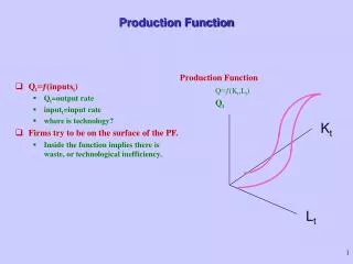
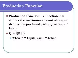
The Production Function II • 1. Costs - short run • measures • relationship - production & costs • 2. Costs - long run • scale expansion path • long run costs • 3. Returns to scale & economies of scale
1. Costs - short run • Fixed & variable costs • fixed = unavoidable • variable = avoidable • Costs rise as output increases • e.g. As L, TPP TC • given PK and PL • inverse relationship MP & MC, AC & AP • Measures of cost - Table 1
Measures of cost • Total costs: TC = TFC + TVC • Average costs: ATC = TC \ TPP • or TC \ Q • ATC = AFC + AVC • Marginal costs: MC =TC \ TPP • ‘…the extra cost of producing one more unit.’ • Shape - Figures 1 to 3
Total costs for firm X Output (Q) 0 1 2 3 4 5 6 7 TVC (£) 0 10 16 21 28 40 60 91 TC (£) 12 22 28 33 40 52 72 103 TFC (£) 12 12 12 12 12 12 12 12 TC TVC TFC fig
Average and marginal physical product b c Output APP MPP Quantity of the variable factor fig
Average and marginal costs MC Costs (£) x fig Output (Q)
2. Costs - long run • K & L are variable • Profit maximisation requires cost minimisation • Choice of technique: if • MPK \ PK > MPL \ PL • 20 \ 2 > 32 \ 8 • 10 > 4
Cost minimisation • i.e. last pound spent on K adds 10 units • Therefore • spend 1 extra pound on K, TPP rises by 10 • spend 2.50 less on L, TPP falls by 10 • output is unchanged, but costs fall 1.50 • Cost minimisation • MPK \ PK = MPL \ PL • tangency of isocost & isoquant
Scale expansion path & long run costs • Vary K & L TPP rises (no. of factories) • See Figure - scale expansion path • Long run average costs • Returns to scale • Scale economies
Deriving an LRAC curve from an isoquant map At an output of 100 LRAC = TC1 / 100 Units of capital (K) 100 O TC1 fig Units of labour (L)
Deriving an LRAC curve from an isoquant map Expansion path Units of capital (K) 700 600 500 400 300 200 100 O TC5 TC1 TC4 TC2 TC3 TC7 TC6 fig Units of labour (L)
A typical long-run average cost curve LRAC Costs O Output fig
Returns to scale • (i) Increasing returns • LRAC • a % increase in inputs leads to a larger % increase in output • economies of scale • (ii) Constant returns • LRAC constant • a given % increase in inputs leads to the same % increase in output
Returns to scale • (iii) Decreasing returns • LRAC • a % increase in inputs leads to a smaller % increase in output • diseconomies of scale • Economies of scale • plant level economies • multi-plant economies • Diseconomies of scale
Conclusion • Cost minimisation - long run • Profit = Revenue - Cost • Profit maximisation - level? • Market structure: • Perfect competition • Monopolistic competition • Oligopoly • Monopoly