Download

1 / 34
340 likes | 473 Views
Example. A toxocologist* conducts an experiment to investigate the relation between PCB (industrial chemical and pollutant) exposure and estrogen production in breast cancer cells. She conducts the following “concentration / response” experiment.

E N D
Example • A toxocologist* conducts an experiment to investigate the relation between PCB (industrial chemical and pollutant) exposure and estrogen production in breast cancer cells. • She conducts the following “concentration / response” experiment. *Following is from the research of Professor Kathleen Arcaro (department of Veterinary and Animal Sciences, Umass)
Picture of a plate There are 48 “wells” on each plate. Breast cancer cells are grown in each 32 of them (darkcircles). 24 of thosewells contain acertain amount of PCB (one of several types ofPCBs). White circles are not part of the experiment. After growth, amachine determinesthe amount of estrogenproduced in each well. Left two columnsare “controls” (no PCB in these wells) Experiment is repeated on 30 plates.
One way to think about the data: Each plate provides one number (we’ll see a better way to analyze the data later): Average Control Cell Estrogenproduction Average Estrogen Produced by cells exposed to PCBs minus Plate Number X1 = 1146.83 X2 = -95.67 X3 = -60.67 X4 = 160.17 X5 = 509.17 etc 516.24 1078.67 1 2 3 4 5 etc X (Overall Mean) S (Overall Std Dev) Summary of all 30 plates.
Less estrogen in PCB exposed cells. More estrogen in PCB exposed cells (relative to controls). Each plate contributesone data point to this histogram. This is an estimate of the distribution of X, not the distribution of X.
Statistical Question: • A x > 0 says that more estrogen is produced by cells that are exposed to PCBs on average. • Observed x = 516.24, but there’s a fair amount of “noise” in the data (s = 1078.67). • Is this x statistically significantly positive?(in other words: If the experiment were repeated, how certain should we be that we’ll see x>0 again?)
To answer the question, we need to know the probability distribution of x In general, the central limit theorem says that the sample mean has a normal distribution (when n>30 or so…) X ~ N(m,s2/n) We don’t know m or s, but we do have estimates: x = 516.24, s = 1078.67 This gives us a good guess at the distribution of X (i.e. A model for how X would behave if we took another sample): X ~ N(516.24, 1078.672/30)
0.0020 Distribution of X-Bar N(516.24,1078.672/30) 0.0015 normal density 0.0010 0.0005 0.0 0 500 1000 X-bar Informally, since 0 is in the “tail” of the distribution of X, then seeing an x < 0 is unlikely (i.e. these PCBs cause estrogen production on average)
More formally:Confidence intervals for the mean • A 1-a% confidence interval for the mean: x +/- za/2s/sqrt(n)x and s are the sample mean and sample std deviation from n observations za/2 = number such that Pr(Z<za/2) = 1-a/2 Rough Interpretation: interval covers “inner” 1-a% of the best guess at x’s distribution
Observed x 95% of the area under the curve 0.0020 Distribution of X 0.0015 normal density 0.0010 0.0005 0.0 0 500 1000 130.44 920.44 X-bar 95% confidence interval (a = 0.05) 516.24 +/- 1.96 (1078.67) / 5.48 516.24 +/- 385.80 = (130.44 , 902.44) x +/- za/2s/sqrt(n)
95% confidence interval for mean estrogen production in cells + PCB – mean production in control cells is (130.44 , 902.44). • Since 0 is not in this interval, there’s “statistically significant” evidence (at 95% confidence) that mean estrogen production is higher for cells plus PCB.
Meaning of 1-a% confidence interval: We can be “1-a% confident” that the true mean is in this interval… Note that theinterval is the randomthing. The true meanis a fixed number.
Order these from narrowest to widest: 90% confidence interval 99% confidence interval 95% confidence interval 80% confidence interval
Ordered from narrowest to widest: Narrowest: 80% confidence interval 90% confidence interval 95% confidence interval Widest: 99% confidence interval Common sense: we can say with high confidence that the mean is somewhere within an extremely wide interval… Math: z0.005 is bigger than z0.1 since the subscriptdescribes a “tail” probability…
za/2 (quick reference) • za/2 is a number such that Pr(-za/2<Z<za/2)=1-a where Z~N(0,1). • Examples: 1-a a/2 za/2 90% 5% 1.64595% 2.5% 1.9699% 0.5% 2.58 Area 1-a 0 -za/2 za/2 Note also: Pr(|Z|<za/2) = 1-a area a/2 area a/2
Observed x 95% of the area under the curve 0.0020 Distribution of X 0.0015 normal density 0.0010 0.0005 0.0 0 500 1000 130.44 920.44 X-bar 95% confidence interval (a = 0.05) 516.24 +/- 1.96 (1078.67) / 5.48 516.24 +/- 385.80 = (130.44 , 902.44) x +/- za/2s/sqrt(n)
A more precise interpretation of the 95% confidence interval Distribution of X-Barwhen mean Is lower limit If true mean is at lower confidencelimit and the experiment is repeated,the probability of seeing the observedx or something larger is 0.025 (=a/2) This interpretation is more precise because the true mean is not random, the data are… 0.0020 0.0015 normal density 0.0010 Area 0.025 (=a/2) 0.0005 0.0 0 516.24 1000 130.44 920.44
Equivalently… Distribution of X-Barwhen mean Is upper limit If true mean is at upper confidencelimit, then if the experiment is repeated,the probability of seeing the observedx or something smaller is 0.025 (=a/2) 0.0020 0.0015 normal density 0.0010 Area 0.025 (=a/2) 0.0005 0.0 0 516.24 1000 920.44
Calculation:Pr( X > observed x when lower limit is true mean)=Pr(X > x) =Pr( (X – lower limit)/(s/sqrt(n)) > (x – lower limit)/(s/sqrt(n))=Pr(Z > [x – (x – za/2s/sqrt(n))]/[s/sqrt(n)] )=Pr(Z > za/2) = a/2 by definition… Observed number Random variable
CONFIDENCE INTERVALS FOR ESTIMATES OF PROPORTIONS • Now that Pedro is healthy, what are your expectations for the Red Sox this season?Will make the playoffs 59% 90 wins 16% 80 wins 14% 70 wins 11% • Number polled (when I took poll) = 81What’s a 90% confidence interval for proportion of people who think they’ll make the playoffs?Is 59% from 81 people significantly greater than ½ (at 90% confidence level?)
Review: The CLT for proportions Let Xi = 1 if person i thinks the Sox will make playoffs. = 0 otherwisewhere i=1,…,81 (indexes people polled). Mean of Xi = pVariance of Xi = p(1-p) p = (X1+…+X81)/81By central limit theorem, P ~ N(p,p(1-p)/n) Xi~Bin(n=1,p)
Confidence Intervals for Proportions • 90% CI for proportion:p +/- z0.10/2sqrt[p*(1-p)/n]0.59 +/- 1.64 sqrt(0.59*0.41/81)0.59 +/- 0.0895[0.505, 0.6795] (uses that p ~ N(p,p(1-p)/n)
Confidence Intervals for Proportions • 90% CI for proportion:p +/- z0.10/2sqrt[p*(1-p)/n]0.59 +/- 1.64 sqrt(0.59*0.41/81)0.59 +/- 0.0895[0.505, 0.6795] In general, a 1-a level confidence interval is:estimator +/- za/2std error(estimator) (uses that p ~ N(p,p(1-p)/n)
p=0.59 Distribution of Pwhen true p = 0.59. 6 Area=0.05 Area=0.05 4 normal density Lower limit0.505 Upper limit0.6795 2 0 0.4 0.5 0.6 0.7 0.8 P-hat
p=0.59 Distribution of Pwhen true p = 0.505. 6 Approximate Area=0.05 4 normal density Lower limit0.505 2 0 0.4 0.5 0.6 0.7 0.8 P-hat
p=0.59 Distribution of Pwhen true p = 0.505. Approximate because Distn of P is N(true p, (true p)(1- true p)/n) 6 True p is in mean and variance Approximate Area=0.05 4 normal density Lower limit0.505 2 0 0.4 0.5 0.6 0.7 0.8 P-hat
If the true p is 0.505, how “rare” is seeing the poll result of 59%? • “Rarity” = Pr( P > 0.59 when true p = 0.505) =Pr[ (P-0.505)/sqrt(.505*.495/81) > (0.59-0.505)/sqrt(.505*.495/81) =Pr( Z > 0.085/0.06) = Pr(Z>1.53) = 0.0630
p=0.59 Distribution of Pwhen true p = 0.505. 6 Area=0.0630 4 normal density Lower limit0.505 2 0 0.4 0.5 0.6 0.7 0.8 P-hat
If the true p is 0.5, how “rare” is seeing and poll result of 59%? • “Rarity” = Pr( P > 0.59 when true p = 0.5) =Pr[ (P-0.5)/sqrt(.5*.5/81) > (0.59-0.5)/sqrt(.5*.5/81) =Pr( Z > 0.09/0.06) = Pr(Z>1.62) = 0.0526 (This is the p-value!)
p=0.59 Distribution of Pwhen true p = 0.5 6 Area=0.0526 4 normal density 0.5 2 0 0.4 0.5 0.6 0.7 0.8 P-hat
Differences between means • Can people discern a difference between Advil and generic ibuprofen on average? • Experiment: “Double Blind Study” • Randomly separate 80 people into two groups of 40 each. • Give one group Advil and generic ibuprofen to the other group. • “Blinding”: person handing out pills and people being tested don’t know which pill they’re getting (pills were dyed). • People report their opinion of how well the pill works (on a scale of 1 to 10). • When we did the experiment, 2 people from the Advil group dropped out. When might this matter?
Results: Advil Group Generic Group 8 6 6 4 4 2 2 0 0 2 4 6 8 10 2 4 6 8 10 score score X Generic = 6.03 S Generic = 2.47 n Generic = 40 X Advil = 6.35 S Advil = 2.32 n Advil = 38 Is X Advil – X Generic = 0.32. Is this“statistically significantly” greater than zero?
In General: 1-a confidence interval is “Estimate +/- za/2 se(estimate)” Variance of X Advil – X Generic is s2Advil /n Advil + s2Generic /n Generic
Variance of X Advil – X Generic is s2Advil /n Advil + s2Generic /n Generic 1-a confidence interval is “Estimate +/- za/2 se(estimate)” When nAdvil and nGeneric are both >30ish, a 1-a confidence interval is XAdvil–XGeneric+/-za/2 sqrt(s2Advil/nAdvil + s2Generic /nGeneric) This is NOT: sAdvil/sqrt(nAdvil) + sGeneric/sqrt(nGeneric)
95% CI for Advil / Generic Example 0.32 +/- 1.96 sqrt(5.38/38 + 6.10/40) = [-0.74,1.38] Can’t claim that people can discern a difference at 95% confidence. Is there a level of confidence at which we could make the claim? Suppose n = 1,000,000. Do you think we could claim a significant difference then?