Download

1 / 20
200 likes | 218 Views
Evolutionary Programming (EP) developed in the 1960s in the USA by D. Fogel is used for machine learning tasks by finite state machines and numerical optimization. EP features a very open framework and self-adaptation of parameters. This overview covers the historical perspective, FSM predictions, modern EP, and application examples like evolving checkers players.

E N D
EP quick overview • Developed: USA in the 1960’s • Early names: D. Fogel • Typically applied to: • traditional EP: machine learning tasks by finite state machines • contemporary EP: (numerical) optimization • Attributed features: • very open framework: any representation and mutation op’s OK • crossbred with ES (contemporary EP) • consequently: hard to say what “standard” EP is • Special: • no recombination • self-adaptation of parameters standard (contemporary EP)
Historical EP perspective • EP aimed at achieving intelligence • Intelligence was viewed as adaptive behaviour • Prediction of the environment was considered a prerequisite to adaptive behaviour • Thus: capability to predict is key to intelligence
Prediction by finite state machines • Finite state machine (FSM): • States S • Inputs I • Outputs O • Transition function : S x I S x O • Transforms input stream into output stream • Can be used for predictions, e.g. to predict next input symbol in a sequence
Vending machine • States: • Got 0 • Got 5p • Got 10p • Inputs: • 5p • 10p • Output: • can of water Vending machine sells water for 15p
FSM example • Consider the FSM with: • S = {A, B, C} • I = {0, 1} • O = {a, b, c} • given by a diagram
FSM as predictor • Consider the following FSM • Task: predict next input • Quality: % of in(i+1) = outi • Given initial state C • Input sequence 011101 • Leads to output 110111 • Quality: 3 out of 5
Introductory example:evolving FSMs to predict primes • P(n) = 1 if n is prime, 0 otherwise • I = N = {1,2,3,…, n, …} • O = {0,1} • Correct prediction: outi= P(in(i+1)) • Fitness function: • 1 point for correct prediction of next input • 0 point for incorrect prediction • Penalty for “too much” states
Introductory example:evolving FSMs to predict primes • Parent selection: each FSM is mutated once • Mutation operators (one selected randomly): • Change an output symbol • Change a state transition (i.e. redirect edge) • Add a state • Delete a state • Change the initial state • Survivor selection: (+) • Results: overfitting, after 202 inputs best FSM had one state and both outputs were 0, i.e., it always predicted “not prime”
Modern EP • No predefined representation in general • Thus: no predefined mutation (must match representation) • Often applies self-adaptation of mutation parameters • In the sequel we present one EP variant, not the canonical EP
Representation • For continuous parameter optimisation • Chromosomes consist of two parts: • Object variables: x1,…,xn • Mutation step sizes: 1,…,n • Full size: x1,…,xn,1,…,n
Mutation • Chromosomes: x1,…,xn,1,…,n • i’ = i•(1 + • N(0,1)) • x’i = xi + i’• Ni(0,1) • 0.2 • boundary rule: ’ < 0 ’ = 0 • Other variants proposed & tried: • Lognormal scheme as in ES • Using variance instead of standard deviation • Mutate -last • Other distributions, e.g, Cauchy instead of Gaussian
Recombination • None • Rationale: one point in the search space stands for a species, not for an individual and there can be no crossover between species • Much historical debate “mutation vs. crossover” • Pragmatic approach seems to prevail today
Parent selection • Each individual creates one child by mutation • Thus: • Deterministic • Not biased by fitness
Survivor selection • P(t): parents, P’(t): offspring • Pairwise competitions in round-robin format: • Each solution x from P(t) P’(t) is evaluated against q other randomly chosen solutions • For each comparison, a "win" is assigned if x is better than its opponent • The solutions with the greatest number of wins are retained to be parents of the next generation • Parameter q allows tuning selection pressure • Typically q = 10
Example application: the Ackley function (Bäck et al ’93) • The Ackley function (here used with n =30): • Representation: • -30 < xi < 30 (coincidence of 30’s!) • 30 variances as step sizes • Mutation with changing object variables first ! • Population size = 200, selection with q = 10 • Termination : after 200000 fitness evaluations • Results: average best solution is 1.4 • 10 –2
Example application: evolving checkers players (Fogel’02) • Neural nets for evaluating future values of moves are evolved • NNs have fixed structure with 5046 weights, these are evolved + one weight for “kings” • Representation: • vector of 5046 real numbers for object variables (weights) • vector of 5046 real numbers for ‘s • Mutation: • Gaussian, lognormal scheme with -first • Plus special mechanism for the kings’ weight • Population size 15
Example application: evolving checkers players (Fogel’02) • Tournament size q = 5 • Programs (with NN inside) play against other programs, no human trainer or hard-wired intelligence • After 840 generation (6 months!) best strategy was tested against humans via Internet • Program earned “expert class” ranking outperforming 99.61% of all rated players
D. B. Fogel, T. J. Hays, S. L. Hahn and J. Quon, "A self-learning evolutionary chess program," in Proceedings of the IEEE, vol. 92, no. 12, pp. 1947-1954, Dec 2004.doi: 10.1109/JPROC.2004.837633 Abstract: A central challenge of artificial intelligence is to create machines that can learn from their own experience and perform at the level of human experts. Using an evolutionary algorithm, a computer program has learned to play chess by playing games against itself. The program learned to evaluate chessboard configurations by using the positions of pieces, material and positional values, and neural networks to assess specific sections of the chessboard. During evolution, the program improved its play by almost 400 rating points. Testing under simulated tournament conditions against Pocket Fritz 2.0 indicated that the evolved program performs above the master level. URL: http://ieeexplore.ieee.org/stamp/stamp.jsp?tp=&arnumber=1360168&isnumber=29834