Download

1 / 53
890 likes | 2.44k Views
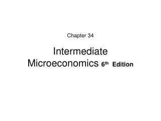
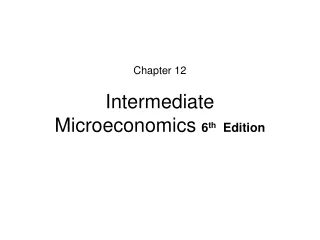
Intermediate Microeconomics and Its Application 9th Edition by Walter Nicholson, Amherst College. Slide Presentation by Mark Karscig Central Missouri State University. © 2004 Thomson Learning/South-Western. Chapter 1. Economic Models. © 2004 Thomson Learning/South-Western.

E N D
Intermediate Microeconomics and Its Application9th EditionbyWalter Nicholson, Amherst College Slide Presentation by Mark Karscig Central Missouri State University © 2004 Thomson Learning/South-Western
Chapter 1 Economic Models © 2004 Thomson Learning/South-Western
What is Microeconomics? • Economics • The study of the allocation of scarce resources among alternative uses • Microeconomics • The study of the economic choices individuals and firms make and how those choices create markets
Economic Models • Simple theoretical descriptions that capture the essentials of how the economy works • Used because the “real world” is too complicated to describe in detail • Models tend to be “unrealistic” but useful • While they fail to show every detail (such as houses on a map) they provide enough structure to solve the problem (such as how a map provides you with a way to solve how to drive to a new location)
The Production Possibility Frontier • A graph showing all possible combinations of goods that can be produced with a fixed amount of resources • Figure 1.1 shows a production possibility frontier where the good goods are food and clothing produced per week • At point A, 10 units of food and 3 units of clothing can be produced
FIGURE 1.1: Production Possibility Frontier Amount of food per week A 10 B 4 0 Amount of clothing per week 3 12
The Production Possibility Frontier • At point B, 4 units of food can be produced and 12 units of clothing • Without more resources, points outside the frontier are unattainable • This demonstrates a basic fact that resources are scarce
Opportunity Cost • The cost of a good or service as measured by the alternative uses that are foregone by producing the good or service
Opportunity Cost Example • As shown in Figure 1.1, if the economy produces one more unit of clothing beyond the 10 that it produces at point A, the amount of food produced decreases by 1/2 from 10 to 9.5 • Thus, the opportunity cost of one unit of clothing is 1/2 unit of food at point A
FIGURE 1.1: Production Possibility Frontier Amount of food per week Opportunity cost of clothing = ½ pound of food A 10 9.5 0 Amount of clothing per week 3 4
Opportunity Cost Example • Figure 1.1 also shows that the opportunity cost of clothing is much higher at point B (1 unit of clothing costs 2 units of food) • The increasing opportunity costs of producing even more clothing is consistent with Ricardo’s and Marshall’s ideas of increasing marginal cost
FIGURE 1.1: Production Possibility Frontier Amount of food per week Opportunity cost of clothing = 2 pounds of food B 4 2 0 Amount of clothing per week 12 13
FIGURE 1.1: Production Possibility Frontier Amount of food per week Opportunity cost of clothing = ½ pound of food A 10 9.5 Opportunity cost of clothing = 2 pounds of food B 4 2 0 Amount of clothing per week 3 4 12 13
APPLICATION 1.1: Do Animals Understand Economics? • Nature provides examples of where animals have scarcity affect their choices • Birds of prey recognize a trade-off between spending time and energy in one area and moving to another location • To avoid using too much energy, animals will leave an area before the food supply is exhausted
Uses of Microeconomics • While the uses of microeconomics are varied, one useful way to categorize is by types of users • Individuals making decisions regarding jobs, purchases, and finances • Businesses making decisions regarding the demand for their product or their costs • Governments making policy decisions regarding laws and regulations
APPLICATION 1.2: Is It Worth Your Time to Be Here? • The typical U.S. college student pays about $18,000 per year in tuition, fees, and room and board charges. One might conclude then, that the “cost” of 4 years of college is about $72,000. • A number of studies have suggested that college graduates earn more than those without such an education.
APPLICATION 1.3: Saving Blockbuster • The largest video rental company incurred a huge financial loss primarily because of the high price of first-run movies • A large part of the “price” of the movie to the customer was not finding the movie in stock. • Blockbuster reached an agreement to guarantee availability and reverse its losses.
APPLICATION 1.4: Microsoft and Antitrust • The central issue of this case is whether or not Microsoft is illegally “monopolizing” various segments of the software industry in violation of the Sherman Antitrust Act. • MIT professor Franklin Fisher suggests that the real danger is allowing Microsoft to dominate the internet browser market which would eliminate competition.
APPLICATION 1.4: Microsoft and Antitrust • MIT professor Richard Schmalensee argues that Microsoft has not acted like a monopoly in the pricing of the Windows operating system • The judge’s decision will have to try to strike a balance between the operating system monopoly and the ability of Microsoft to be innovative
The Basic Supply-Demand Model • A model describing how a good’s price is determined by the behavior of the individual’s who buy the good and the firms that sell it. • Economists argue that market behavior can generally be explained by this model that captures the relationship between consumers’ preferences and firms’ costs.
Adam Smith and the Invisible Hand • Adam Smith (1723-1790) saw prices as the force that directed resources into activities where they were most valuable • Prices told both consumers and firms the “worth” of the good. • Smith’s somewhat incomplete explanation for prices was that they were determined by the costs to produce the goods.
Adam Smith and the Invisible Hand • Since labor was the primary resource used, this led Smith to embrace a labor-based theory of prices. • If catching deer took twice as long as catching a beaver, one deer should trade for two beaver (the relative price of a deer is two beaver’s). • In Figure 1.1(a), the horizontal line at P* shows that any number of deer can be produced without affecting the relative cost
FIGURE 1.2(a): Smith’s Model Price P* Quantity per week
David Ricardo and Diminishing Returns • David Ricardo (1772-1823) believed that labor and other costs would rise with the level of production • for example, as new less fertile land was cultivated, it would require more labor • This increasing cost argument is now referred to as the law of diminishing returns
David Ricardo and Diminishing Returns • The relative price of a good could be practically any amount, depending upon how much was produced • The level of production represented the quantity the country needed to survive • In Figure 1.2(b), as the needs of the country increase from Q1 to Q2 prices increase from P1 to P2
FIGURE 1.2(b): Ricardo’s Model Price P1 Q1 Quantity per week
FIGURE 1.2(b): Ricardo’s Model Price P2 P1 Q1 Q2 Quantity per week
FIGURE 1.2: Early Views of Price Determination Price Price P2 P* P1 Quantity per week Q1 Q2 Quantity per week (a) Smith model ’ (b) Ricardo model ’
Marginalism and Marshall’s Model of Supply and Demand • Ricardo’s model was unable to explain the fall in the relative prices of good during the nineteenth century so a more general model was needed • Economists argued the willingness of people to pay for a good will decline as they have more of it
Marginalism and Marshall’s Model of Supply and Demand • People will be willing to consume more of a good only if the price is lower • The focus of the model was on the value of the last, or marginal, unit purchased • Alfred Marshall (1842-1924) showed how the forces of demand and supply simultaneously determined price
Marginalism and Marshall’s Model of Supply and Demand • In Figure 1.3, the amount of a good purchased per period is shown on the horizontal axis and the price of the good is shown on the vertical axis • The demand curve shows the amount people want to buy at each price and is negatively sloped reflecting the marginalism principle
Marginalism and Marshall’s Model of Supply and Demand • The upward sloping supply curve reflects the idea of increasing cost of making one more unit of a good as total production increases • Supply reflects increasing marginal costs and demand reflects decreasing marginal usefulness
FIGURE 1.3: The Marshall Supply-Demand Cross Price Supply Demand 0 Quantity per week
Market Equilibrium • In Figure 1.3, the demand and supply curve intersect at the market equilibrium point P*, Q* • P* is the equilibrium price: The price at which the quantity demanded by buyers of a good is equal to the quantity supplied by sellers of the good
FIGURE 1.3: The Marshall Supply-Demand Cross Price Demand Supply . Equilibrium point P* 0 Quantity per week Q*
Market Equilibrium • Both demanders and suppliers are satisfied at this price, so there is no incentive for either to alter their behavior unless something else happens • Marshall compared the roles of supply and demand in establishing market equilibrium to the two blades of a pair of scissors working together in order to make a cut
Nonequilibrium Outcomes • If something causes the price to be set above P*, demanders would wish to buy less than Q* while suppliers would produce more than Q* • If something causes the price to be set below P*, demanders would wish to buy more than Q* while suppliers would produce less than Q*
Change in Market Equilibrium: Increased Demand • Figure 1.4 shows the case where people’s demand for the good increases as represented by the shift of the demand curve from D to D’ • A new equilibrium is established where the equilibrium price has increased to P**
FIGURE 1.4: An increase in Demand Alters Equilibrium Price and Quantity D S Price P* Q* Quantity per week 0
FIGURE 1.4: An increase in Demand Alters Equilibrium Price and Quantity D’ S Price D P** P* Q* Q** Quantity per week 0
Change in Market Equilibrium: decrease in Supply • In Figure 1.5 the supply curve has shifted leftward reflecting a decrease in supply brought about because of an increase in supplier costs (say an increase in wages) • At the new equilibrium price P** consumers respond by reducing quantity demanded along the Demand curve D
FIGURE 1.5: A shift in Supply Alters Equilibrium Price and Quantity S Price P* D Q* 0 Quantity per week
FIGURE 1.5: A shift in Supply Alters Equilibrium Price and Quantity S’ Price S P** P* D Q** Q* 0 Quantity per week
How Economists Verify Theoretical Models • Two methods are used • Testing Assumptions: Verifying economic models by examining validity of the assumptions on which they are based • Testing Predictions: Verifying economic models by asking if they can accurately predict real-world events
Testing Assumptions • One approach would be to determine if the assumptions are reasonable • The obvious problem is that people have differing opinion regarding reasonable • Empirical evidence can also be used • Results of such methods have had problems similar to those found in opinion polls
Testing Predictions • Economists, such as Milton Friedman argue that all theories require unrealistic assumptions • The theory is only useful if it can be used to predict real-world events • Even if firms state they don’t maximize profits, if their behavior can be predicted by using this assumption, the theory is useful
Models of Many Markets • Marshall's model of supply and demand is a partial equilibrium model: An economic model of a single market • To show the effects of a change in one market on others requires a general equilibrium model: An economic model of a complete system of markets
APPLICATION 1.5: Economics According to Bono • The Spring 2002 trip to Africa by the Irish rock star Bono and U.S. Treasury Secretary Paul O’Neill sparked much interesting dialogue about economics • Bono claimed that recently enacted agricultural subsidies in the U.S. were harming struggling farmers in Africa
APPLICATION 1.5: Economics According to Bono • In Figure 1 U.S. farm subsidies reduce the world price of this crop from P* to P**. • Exports from this African country fall from QS – QD to Q’S – Q’D
Figure 1: U.S. Subsidies Reduce African Exports P S P* P** D QD Q’D Q’S QS Q