Download
1 / 23
240 likes | 553 Views
Predation – Chapter 13. Types of Predators. Herbivores – animals that prey on green plants or their seed and fruits. Plants are usually damaged but not killed Carnivores – animals that eat herbivores or other carnivores.

E N D
Types of Predators • Herbivores – animals that prey on green plants or their seed and fruits. • Plants are usually damaged but not killed • Carnivores – animals that eat herbivores or other carnivores. • Insect Parasitoids – lay eggs on or near host insect, which is subsequently killed and eaten. • Phorid fly • Parasites – plants or animals that live on or in their hosts and depend on their host for nutrition. • Cannibalism – predator and prey are the same species
P1 P2 P1 P2 H H1 H2 Predators can interact with one another by competition. Predator populations may also be affected by indirect effects. Indirect Competition via exploitation competition Indirect Competition without competition
Three Important Predation Processes • Predation on a population may restrict distribution or abundance of the prey • If affected animal is pest – then good • If affected animal is valuable – then bad • Predation is another major type of interaction (like competition) that can influence the organization of communities. • Predation is a major selective force. • Many adaptations we see in organisms, such as warning coloration, have their explanation in predator-prey coevolution
Mathematical Models of Predation – discrete generations Small prey population will increase without predation according to: Nt+1 = [1.0 – B(zt)]Nt If prey abundance is determined by predator abundance, then the whole predator population must eat proportionately more prey when prey densities are high. We can subtract a term from the above equation: Nt+1 = [1.0 – B(zt)]Nt - CNtPt Accounts for predation Pt = population size of predators in generation t C = a constant measuring the efficiency of the predator
Predator Population Growth If we assume that the reproductive rate of predators is dependent on prey abundance, then: Pt+1 = QNtPt Pt= population size of predator N = population size of prey t = generation number Q = a constant measuring the efficiency of utilization of prey for reproduction for predators
Nt+1 R = = [1.0 – B(Neq)] Nt Pt+1 or S = = QNeq Pt With predators absent and population low, prey growth is approximated by: Nt+1 = [1.0 – B(Neq)]Nt Rearrange equation: R= maximum finite rate of prey population increase When prey are at equilibrium and predators are scarce, predator growth is approximated by: S= maximum finite rate of predator population increase Pt+1 = QNtPt
2 = Q(100) Q= 0.02 S = QNeq For Predator; If S = 2: ThenPt+1= 0.02NtPt Predator population size Example: For Prey; If R = 1.5; Neq = 100; absolute vale of B = 0.005; C = 0.5: Nt+1 = [1.0 – B(zt)]Nt - CNtPt Nt+1 = [1.0 – 0.005(zt)]Nt – 0.5NtPt Prey population size We predict a predator-prey population cycle
Lynx and Snowshoe Hare • Both lynx and snowshoe hare populations oscillate through a 9-year period.
How Do Predators Respond to a Change in Prey Density? • Numerical Response – an increase in number due to an increase in reproduction. • Aggregative Response – Predators tend to aggregate where the prey is at a high density. • Functional Response – the number of prey eaten by an individual predator increases as the number of prey increases. • Developmental Response – individual predators eat more or fewer prey as the predator grows.
Aggregate Response Predators tend to aggregate where the prey is at a high density:
Three Functional Responses Type 1 – Prey consumed increases with prey density. Type 2 – Prey consumed increases rapidly with prey density, then levels off. Type 3 – Prey consumed follows a logistic pattern as prey density increases.
Optimal Foraging Theory-predicting behavior of predators in choosing prey • Assume the predator makes a conscience decision when selecting prey when simultaneously faced with two or more choices. • Assume the predator will maximize the net rate of energy gain while foraging. • More energy is better for the predator because it will be able to meet its metabolic demands and still have energy for: • Defending a territory • Fighting • Reproducing • Moving
Energy value E Handling Time h Profitability = = Maximizing Daily Energy Uptake • Search time – the time it takes a predator to search for a prey. • Handling time – the time it takes a predator to kill and eat a single prey. • Energy Value – the amount of energy available to the predator from the prey. • Profitability – the amount of surplus energy a predator gets from a prey:
E1 E2 > h1 h2 If a predator has two prey types to choose from. Prey 1 is large and has a greater handling time than the smaller prey 2. However, assume the profitability is greater for prey 1, such that: • If a predator encounters a prey it must decide to eat it or ignore it. Two rules: • If the predator encounters prey 1, it should always eat it because it is the most profitable. • If it encounters prey 2, it should eat it if the gain from eating it exceeds the gain from rejecting it and searching for a more profitable prey 1.
E1 > E2 S1 + h1 h2 Define S1 as the average search time to find a prey 1 individual then: This model suggests that a predator will consume prey species 2 if the search time for prey 1 is large (energetically costly). Predators will maximize profitability.
Size of Prey-Optimal Foraging Theory • Predators tend to eat medium size prey • If the prey is too small, the energy value is not great enough even though the handling time is small • If the prey is too large, the handling time may be so great that it consumes too much of the prey’s energy value • Medium size prey have maximum profitability
Generalists predators tend to stabilize prey numbers • Once a prey population gets too small, the predator will feed on something else • If a prey population becomes very abundant, predators will feed on them • Specialist predators tend to cause instability in prey numbers • Because a specialists feeds on only one species, the predator-prey populations tend to oscillate (lynx-snowshoe hare).
Evolution of Predator-Prey Systems • Coevolution – evolutionary change in two or more interacting species. • For this chapter, the coevolution of predator and prey • Prey that are best able to escape predators are strongly selected for. • Those that get caught die • Predators that are better able to catch prey are selected for. • If a predator misses a prey, it only loses its meal, not its life
Do Predators Only Eat The Weak? Evaluation of prey quality in predation by a trained red-tailed hawk. Predators do tend to capture more substandard prey of difficult to catch species, but not necessarily easy to catch species.
Anti-predator Defense Strategies • Warning Coloration – widespread correlation between conspicuous coloration (usually red or some other bright color) and the presence of aversive qualities. • If a predator samples one from a group and decides that it is not a good prey, then the rest are protected. • Some prey species have evolved to mimic dangerous animals • Group Living – Safety in numbers. • More eyes can lead to early detection of predators. • If prey are not much smaller than predator, the prey can gang-up on the predator. • Predator may become confused when the prey group flees in several directions.