Download
1 / 47
500 likes | 561 Views
This agenda covers the fundamentals of nearest neighbor techniques in artificial intelligence, focusing on applications like robotic motion and credit rating. It delves into efficient implementations using k-d trees and parallelism, discusses extensions, limitations, and implementation challenges. Examples illustrate how nearest neighbor methods work, from modeling robotic motion to credit rating classification. The agenda also explores efficient implementations and the importance of proper distance measures. Further topics include vector space models, text classification, information retrieval phases, and models for retrieval and classification using the Vector Space Model.

E N D
Nearest Neighbor &Information Retrieval Search Artificial Intelligence CMSC 25000 January 29, 2004
Agenda • Machine learning: Introduction • Nearest neighbor techniques • Applications: Robotic motion, Credit rating • Information retrieval search • Efficient implementations: • k-d trees, parallelism • Extensions: K-nearest neighbor • Limitations: • Distance, dimensions, & irrelevant attributes
Nearest Neighbor • Memory- or case- based learning • Supervised method: Training • Record labeled instances and feature-value vectors • For each new, unlabeled instance • Identify “nearest” labeled instance • Assign same label • Consistency heuristic: Assume that a property is the same as that of the nearest reference case.
Nearest Neighbor Example • Problem: Robot arm motion • Difficult to model analytically • Kinematic equations • Relate joint angles and manipulator positions • Dynamics equations • Relate motor torques to joint angles • Difficult to achieve good results modeling robotic arms or human arm • Many factors & measurements
Nearest Neighbor Example • Solution: • Move robot arm around • Record parameters and trajectory segment • Table: torques, positions,velocities, squared velocities, velocity products, accelerations • To follow a new path: • Break into segments • Find closest segments in table • Get those torques (interpolate as necessary)
Nearest Neighbor Example • Issue: Big table • First time with new trajectory • “Closest” isn’t close • Table is sparse - few entries • Solution: Practice • As attempt trajectory, fill in more of table • After few attempts, very close
Nearest Neighbor Example II • Credit Rating: • Classifier: Good / Poor • Features: • L = # late payments/yr; • R = Income/Expenses Name L R G/P A 0 1.2 G B 25 0.4 P C 5 0.7 G D 20 0.8 P E 30 0.85 P F 11 1.2 G G 7 1.15 G H 15 0.8 P
Nearest Neighbor Example II Name L R G/P A 0 1.2 G A F B 25 0.4 P 1 G R E C 5 0.7 G H D C D 20 0.8 P E 30 0.85 P B F 11 1.2 G G 7 1.15 G 10 20 30 L H 15 0.8 P
Nearest Neighbor Example II Name L R G/P I 6 1.15 G A F K J 22 0.45 P 1 I G ?? E K 15 1.2 D H R C J B Distance Measure: Sqrt ((L1-L2)^2 + [sqrt(10)*(R1-R2)]^2)) - Scaled distance 10 20 30 L
Efficient Implementations • Classification cost: • Find nearest neighbor: O(n) • Compute distance between unknown and all instances • Compare distances • Problematic for large data sets • Alternative: • Use binary search to reduce to O(log n)
Roadmap • Problem: • Matching Topics and Documents • Methods: • Classic: Vector Space Model • Challenge I: Beyond literal matching • Expansion Strategies • Challenge II: Authoritative source • Page Rank • Hubs & Authorities
Matching Topics and Documents • Two main perspectives: • Pre-defined, fixed, finite topics: • “Text Classification” • Arbitrary topics, typically defined by statement of information need (aka query) • “Information Retrieval”
Three Steps to IR • Three phases: • Indexing: Build collection of document representations • Query construction: • Convert query text to vector • Retrieval: • Compute similarity between query and doc representation • Return closest match
Matching Topics and Documents • Documents are “about” some topic(s) • Question: Evidence of “aboutness”? • Words !! • Possibly also meta-data in documents • Tags, etc • Model encodes how words capture topic • E.g. “Bag of words” model, Boolean matching • What information is captured? • How is similarity computed?
Models for Retrieval and Classification • Plethora of models are used • Here: • Vector Space Model
Vector Space Information Retrieval • Task: • Document collection • Query specifies information need: free text • Relevance judgments: 0/1 for all docs • Word evidence: Bag of words • No ordering information
Vector Space Model Tv Program Computer Two documents: computer program, tv program Query: computer program : matches 1 st doc: exact: distance=2 vs 0 educational program: matches both equally: distance=1
Vector Space Model • Represent documents and queries as • Vectors of term-based features • Features: tied to occurrence of terms in collection • E.g. • Solution 1: Binary features: t=1 if present, 0 otherwise • Similiarity: number of terms in common • Dot product
Question • What’s wrong with this?
Vector Space Model II • Problem: Not all terms equally interesting • E.g. the vs dog vs Levow • Solution: Replace binary term features with weights • Document collection: term-by-document matrix • View as vector in multidimensional space • Nearby vectors are related • Normalize for vector length
Vector Similarity Computation • Similarity = Dot product • Normalization: • Normalize weights in advance • Normalize post-hoc
Term Weighting • “Aboutness” • To what degree is this term what document is about? • Within document measure • Term frequency (tf): # occurrences of t in doc j • “Specificity” • How surprised are you to see this term? • Collection frequency • Inverse document frequency (idf):
Term Selection & Formation • Selection: • Some terms are truly useless • Too frequent, no content • E.g. the, a, and,… • Stop words: ignore such terms altogether • Creation: • Too many surface forms for same concepts • E.g. inflections of words: verb conjugations, plural • Stem terms: treat all forms as same underlying
Key Issue • All approaches operate on term matching • If a synonym, rather than original term, is used, approach fails • Develop more robust techniques • Match “concept” rather than term • Expansion approaches • Add in related terms to enhance matching • Mapping techniques • Associate terms to concepts • Aspect models, stemming
Expansion Techniques • Can apply to query or document • Thesaurus expansion • Use linguistic resource – thesaurus, WordNet – to add synonyms/related terms • Feedback expansion • Add terms that “should have appeared” • User interaction • Direct or relevance feedback • Automatic pseudo relevance feedback
Query Refinement • Typical queries very short, ambiguous • Cat: animal/Unix command • Add more terms to disambiguate, improve • Relevance feedback • Retrieve with original queries • Present results • Ask user to tag relevant/non-relevant • “push” toward relevant vectors, away from nr • β+γ=1 (0.75,0.25); r: rel docs, s: non-rel docs • “Roccio” expansion formula
Compression Techniques • Reduce surface term variation to concepts • Stemming • Map inflectional variants to root • E.g. see, sees, seen, saw -> see • Crucial for highly inflected languages – Czech, Arabic • Aspect models • Matrix representations typically very sparse • Reduce dimensionality to small # key aspects • Mapping contextually similar terms together • Latent semantic analysis
Authoritative Sources • Based on vector space alone, what would you expect to get searching for “search engine”? • Would you expect to get Google?
Issue Text isn’t always best indicator of content Example: • “search engine” • Text search -> review of search engines • Term doesn’t appear on search engine pages • Term probably appears on many pages that point to many search engines
Hubs & Authorities • Not all sites are created equal • Finding “better” sites • Question: What defines a good site? • Authoritative • Not just content, but connections! • One that many other sites think is good • Site that is pointed to by many other sites • Authority
Conferring Authority • Authorities rarely link to each other • Competition • Hubs: • Relevant sites point to prominent sites on topic • Often not prominent themselves • Professional or amateur • Good Hubs Good Authorities
Computing HITS • Finding Hubs and Authorities • Two steps: • Sampling: • Find potential authorities • Weight-propagation: • Iteratively estimate best hubs and authorities
Sampling • Identify potential hubs and authorities • Connected subsections of web • Select root set with standard text query • Construct base set: • All nodes pointed to by root set • All nodes that point to root set • Drop within-domain links • 1000-5000 pages
Weight-propagation • Weights: • Authority weight: • Hub weight: • All weights are relative • Updating: • Converges • Pages with high x: good authorities; y: good hubs
Google’s PageRank • Identifies authorities • Important pages are those pointed to by many other pages • Better pointers, higher rank • Ranks search results • t:page pointing to A; C(t): number of outbound links • d:damping measure • Actual ranking on logarithmic scale • Iterate
Contrasts • Internal links • Large sites carry more weight • If well-designed • H&A ignores site-internals • Outbound links explicitly penalized • Lots of tweaks….
Web Search • Search by content • Vector space model • Word-based representation • “Aboutness” and “Surprise” • Enhancing matches • Simple learning model • Search by structure • Authorities identified by link structure of web • Hubs confer authority
Efficient Implementation: K-D Trees • Divide instances into sets based on features • Binary branching: E.g. > value • 2^d leaves with d split path = n • d= O(log n) • To split cases into sets, • If there is one element in the set, stop • Otherwise pick a feature to split on • Find average position of two middle objects on that dimension • Split remaining objects based on average position • Recursively split subsets
R > 0.825? L > 17.5? L > 9 ? R > 0.6? R > 0.75? R > 1.175 ? R > 1.025 ? K-D Trees: Classification Yes No No Yes Yes No No Yes No Yes No No Yes Yes Poor Good Good Poor Good Good Poor Good
Efficient Implementation:Parallel Hardware • Classification cost: • # distance computations • Const time if O(n) processors • Cost of finding closest • Compute pairwise minimum, successively • O(log n) time
Nearest Neighbor: Issues • Prediction can be expensive if many features • Affected by classification, feature noise • One entry can change prediction • Definition of distance metric • How to combine different features • Different types, ranges of values • Sensitive to feature selection
Nearest Neighbor Analysis • Problem: • Ambiguous labeling, Training Noise • Solution: • K-nearest neighbors • Not just single nearest instance • Compare to K nearest neighbors • Label according to majority of K • What should K be? • Often 3, can train as well
Nearest Neighbor: Analysis • Issue: • What is a good distance metric? • How should features be combined? • Strategy: • (Typically weighted) Euclidean distance • Feature scaling: Normalization • Good starting point: • (Feature - Feature_mean)/Feature_standard_deviation • Rescales all values - Centered on 0 with std_dev 1
Nearest Neighbor: Analysis • Issue: • What features should we use? • E.g. Credit rating: Many possible features • Tax bracket, debt burden, retirement savings, etc.. • Nearest neighbor uses ALL • Irrelevant feature(s) could mislead • Fundamental problem with nearest neighbor
Nearest Neighbor: Advantages • Fast training: • Just record feature vector - output value set • Can model wide variety of functions • Complex decision boundaries • Weak inductive bias • Very generally applicable
Summary • Machine learning: • Acquire function from input features to value • Based on prior training instances • Supervised vs Unsupervised learning • Classification and Regression • Inductive bias: • Representation of function to learn • Complexity, Generalization, & Validation
Summary: Nearest Neighbor • Nearest neighbor: • Training: record input vectors + output value • Prediction: closest training instance to new data • Efficient implementations • Pros: fast training, very general, little bias • Cons: distance metric (scaling), sensitivity to noise & extraneous features