Download

1 / 42
420 likes | 888 Views
Malware clustering and classification. Peng Li pengli@cs.unc.edu. 3 Papers. “Behavioral Classification”. T. Lee and J. J. Mody . In EICAR (European Institute for Computer Antivirus Research) Conference, 2006. “Learning and Classification of Malware Behavior”.

E N D
Malware clustering and classification Peng Li pengli@cs.unc.edu
3 Papers • “Behavioral Classification”. T. Lee and J. J. Mody. In EICAR (European Institute for Computer Antivirus Research) Conference, 2006. • “Learning and Classification of Malware Behavior”. KonradRieck, Thorsten Holz, CarstenWillems, Patrick Düssel, PavelLaskov. In Fifth. Conference on Detection of Intrusions and Malware & Vulnerability Assessment (DIMVA 08) • “Scalable, Behavior-Based Malware Clustering”. Ulrich Bayer, Paolo Milani Comparetti, Clemens Hlauschek, Christopher Kruegel, and Engin Kirda. In Proceedings of the Network and Distributed System Security Symposium (NDSS’09), San Diego, California, USA, February 2009
Malware • Malware, short for malicious software, is software designed to infiltrate or damage a computer system without the owner's informed consent. • Viruses (infecting) and worms (propagating) • Trojan horses (inviting), rootkits (hiding), and backdoors (accessing) • Spyware (commercial), botnets (chat channel), keystroke loggers (logging), etc
Battles between malware and defenses • Malware development: • Encryption; (payload encrypted) • Polymorphism; (payload encrypted, varying keys) • Metamorphism; (diff instructions, same functionality) • Obfuscation; (semantics preserving) • Defenses: • Scanner; (static, on binary to detect pattern) • Emulator; (dynamic execution) • Heuristics; [Polychronakis, 07]
Malware variants • Encrypted; • Polymorphic; • Metamorphic; • Obfuscated; http://www.pandasecurity.pk/collective_intelligence.php
Invariants in malware • Code re-use; • Byte stream; • Opcode sequence; • Instruction sequence; • Same semantics; • System Call; • API Call; • System Objects Changes;
Malware Classification • Effectively capture knowledge of the malware to represent; • The representation can enable classifiers to efficiently and effectively correlate data across large number of objects. • Malicious software is classified into families, each family originating from a single source base and exhibiting a set of consistent behaviors.
Static Analysis vs. Runtime Analysis • Static Analysis (source code or binary) • Bytes; • Tokens; • Instructions; • Basic Block; • CFG and CG; • Runtime Analysis (emulator) • Instructions; • Basic Blocks; • System calls; • API calls; • System object dynamics;
Representations • Sets; • Sequences; Edit distance, hamming distance, etc • Feature vectors; SVM
Behavioral Classification T. Lee and J. J. Mody. In EICAR (European Institute for Computer Antivirus Research) Conference, 2006.
Roadmap • Events are recorded and ordered (by time); • Format events; • Compute (pairwise) Levenshtein Distance (string edit distance) on sequences of events; • Do K-medoid clustering; • Do Nearest Neighbor classification.
Event Formalization • To capture rich behavior semantics, each event contains the following information • Event ID • Event object (e.g registry, file, process, socket, etc.) • Event subject if applicable (i.e. the process that takes the action) • Kernel function called if applicable • Action parameters (e.g. registry value, file path, IP address) • Status of the action (e.g. file handle created, registry removed, etc.) • For example, a registry open key event will look like this,
Levenshtein Distance • Operation = Op (Event) • Operations include but not limited to • Insert (Event) • Remove (Event) • Replace (Event1, Event2) • The cost of a transformation from one event sequence to another is defined by the cost of applying an ordered set of operations required to complete the transformation. Cost (Transformation) = ΣiCost (Operationi) • The distance between two event sequence is therefore minimum cost incurred by one of the transformations. (Dynamic programming using a m*n matrix)
Evaluation Sample Sets:
Setting up • Randomly, 90% of data for training and 10% for testing • K (# of clusters) is set to the multiples of the number of families in the dataset (m) from 1 to 4 (i.e. k = m, 2*m, 3*m and 4*m). E (max # of events) is set to 100, 500 and 1000. • Two metrics for evaluations: • Error rate: ER = number of incorrectly classified samples / total number of samples. Accuracy is defined as AC = 1 – ER • Accuracy Gain of x over y is defined as G(x,y) = | (ER(y) – ER(x))/ER(x) |
Results Experiment A: Experiment B:
Results • Accuracy vs. #ClustersError rate reduces as number of clusters increase. • Accuracy vs. Maximum #EventsError rate reduces as the event cap increases, because the more events we observe, the more accurately we can capture the behavior of the malware. • Accuracy Gain vs. Number of EventsThe gain in accuracy is more substantial at lower event caps (100 vs. 500) than at higher event caps (500 vs. 1000), which indicates that between 100 to 500 events, the clustering had most of the information it needs to form good quality clusters. • Accuracy vs. Number of FamiliesThe 11-family experiment outperforms in accuracy the 3-family experiment in high event cap tests (1000), but the result is opposite in lower event cap tests (100). As we investigate further, we found that the same outliers were found in both experiments, and because there were more semantic clusters (11 vs. 3), the outlier effects were contained.
Learning and Classification of Malware BehaviorKonradRieck, Thorsten Holz, CarstenWillems, Patrick Düssel, PavelLaskov.In Fifth. Conference on Detection of Intrusions and Malware & Vulnerability Assessment (DIMVA 08)
Compared to paper 1 • Both obtain traces dynamically; • Different representation of events; • Paper 1: structure • Paper 2: strings directly from API • Different organization of events; • Paper 1: sequences • Paper 2: strings as features 4. Different classification techniques;
Feature vector from report • A document – in our case an analysis report – is characterized by frequencies of contained strings. • All reports X; • The set of considered strings as feature set F; • Take • We derive an embedding function which maps analysis report to an |F|-dimensional vector space by considering the frequencies of all strings in F: |F|
SVM The optimal hyperplane is represented by a vector w and a scalar b such that the inner product of w with vectors (yi) of the two classes are separated by an interval between -1 and +1 subject to b: Kernel function: SVM classifies a new report x :
Multi-class • Maximum distance. A label is assigned to a new behavior report by choosing the classifier with the highest positive score, reflecting the distance to the most discriminative hyperplane. • Maximum probability estimate. Additional calibration of the outputs of SVM classifiers allows to interpret them as probability estimates. Under some mild probabilistic assumptions, the conditional posterior probability of the class +1 can be expressed as: where the parameters A and B are estimated by a logistic regression fit on an independent training data set. Using these probability estimates, we choose the malware family with the highest estimate as our classification result.
Setting up • The malware corpus of 10,072 samples is randomly split into three partitions, a training, validation and testing partition. (labeled by AviraAntiVir) • The training partition is used to learn individual SVM classifiers for each of the 14 malware families using different parameters for regularization and kernel functions. The best classifier for each malware family is then selected using the classification accuracy obtained on the validation partition. • Finally, the overall performance is measured using the combined classifier (maximum distance) on the testing partition.
Experiment 1(general) Maximal distance as the multi-class classifier.
Experiment 2 (prediction) Maximal distance as the multi-class classifier.
Experiment 3(unknown behavior) Instead of using the maximum distance to determine the current family we consider probability estimatesfor each family. i.e. Given a malware sample, we now require exactly one SVM classifier to yield a probability estimate larger 50% and reject all other cases as unknown behavior. All using extended classifier for the following sub-experiments: Sub-experiment 1: using the same testing set as in experiment 1; Sub-experiment 2: using 530 samples not contained in the learning corpus; Sub-experiment 3: using 498 benign binaries;
Experiment 3(unknown behavior) For sub-experiment 1, accuracy dropped from 88% to 76% but with strong confidence For sub-experiment 3, not shown here, all reports are assigned to unknown.
Scalable, Behavior-Based Malware Clustering Ulrich Bayer, Paolo Milani Comparetti, Clemens Hlauschek, Christopher Kruegel, and Engin Kirda In Proceedings of the Network and Distributed System Security Symposium (NDSS’09), San Diego, California, USA, February 2009
Compared to paper 1&2 • Also collecting traces dynamically; • In addition to the info collected for paper 1 & 2, they also do system call monitoring and do data flow and control flow dependency analysis; (e.g. a random filename is associated with a source of random; user intended cmp or not) • Scalable clustering using LSH; • Unsupervised learning, to facilitate manually malware classification process on a large data set.
Profiles to features • As mentioned previously, a behavioral profile captures the operations of a program at a higher level of abstraction. To this end, we model a sample’s behavior in the form of OS objects, operations that are carried out on these objects, dependences between OS objects and comparisons between OS objects.
Approximation of all near pairs using LSH • Jaccard index as a measure of similarity between two samples a and b, defined as • Given a similarity threshold t, we employ the LSH algorithm (Property: Pr[h(a) = h(b)] = similarity(a, b)) to compute a set S which approximates the set T of all near pairs in A × A, defined as • Refining: for each pair a, b in S, we compute the similarity J(a, b) and discard the pair if J(a, b) < t
Hierarchical clustering Then, we sort the remaining pairs in S by similarity. This allows to produce an approximate, single-linkage hierarchical clustering of A, up to the threshold value t. Single-linkage clustering: distance between groups = distance between the closest pair of objects
Setting up • First, obtained a set of 14,212 malware samples that were submitted to ANUBIS in the period from October 27, 2007 to January 31, 2008. • Then, scanned each sample with 6 different anti-virus programs. For the initial reference clustering, we selected only those samples for which the majority of the anti-virus programs reported the same malware family (this required us to define a mapping between the different labels that are used by different anti-virus products). This resulted in a total of 2,658 samples.
Comparing clusterings Example: Testing clustering: 1 ||2, 3, 4, 5, 6, 7, 8, 9, 10 Precision: 1 + 5 = 6 Recall: 4 + 5 = 10 Reference clustering: 1, 2, 3, 4, 5 || 6, 7, 8, 9, 10
Evaluation • Our system produced 87 clusters, while the reference clustering consists of 84 clusters. For our results, we derived a precision of 0.984 and a recall of 0.930 (t = 0.7)