Download

1 / 49
490 likes | 508 Views
Explore hierarchical cluster analysis including agglomerative & divisive methods, proximity matrix, inter-cluster similarity, and common techniques in data clustering.

E N D
Cluster Analysis • What is Cluster Analysis? • Types of Data in Cluster Analysis • A Categorization of Major Clustering Methods • Partitioning Methods • Hierarchical Methods • Density-Based Methods • Grid-Based Methods • Model-Based Clustering Methods • Outlier Analysis • Summary
Hierarchical Clustering • Produces a set of nested clusters organized as a hierarchical tree • Can be visualized as a dendrogram • A tree like diagram that records the sequences of merges or splits
Strengths of Hierarchical Clustering • Do not have to assume any particular number of clusters • Any desired number of clusters can be obtained by ‘cutting’ the dendogram at the proper level • They may correspond to meaningful taxonomies • Example in biological sciences (e.g., animal kingdom, phylogeny reconstruction, …)
Hierarchical Clustering • Two main types of hierarchical clustering • Agglomerative: • Start with the points as individual clusters • At each step, merge the closest pair of clusters until only one cluster (or k clusters) left • Divisive: • Start with one, all-inclusive cluster • At each step, split a cluster until each cluster contains a point (or there are k clusters) • Traditional hierarchical algorithms use a similarity or distance matrix • Merge or split one cluster at a time
Agglomerative Clustering Algorithm • More popular hierarchical clustering technique • Basic algorithm is straightforward • Compute the proximity matrix • Let each data point be a cluster • Repeat • Merge the two closest clusters • Update the proximity matrix • Until only a single cluster remains • Key operation is the computation of the proximity of two clusters • Different approaches to defining the distance between clusters distinguish the different algorithms
p1 p2 p3 p4 p5 . . . p1 p2 p3 p4 p5 . . . Starting Situation • Start with clusters of individual points and a proximity matrix Proximity Matrix
C1 C2 C3 C4 C5 C1 C2 C3 C4 C5 Intermediate Situation • After some merging steps, we have some clusters C3 C4 Proximity Matrix C1 C5 C2
C1 C2 C3 C4 C5 C1 C2 C3 C4 C5 Intermediate Situation • We want to merge the two closest clusters (C2 and C5) and update the proximity matrix. C3 C4 Proximity Matrix C1 C5 C2
After Merging C2 U C5 • The question is “How do we update the proximity matrix?” C1 C3 C4 C1 ? ? ? ? ? C2 U C5 C3 C3 ? C4 ? C4 Proximity Matrix C1 C2 U C5
p1 p2 p3 p4 p5 . . . p1 p2 p3 p4 p5 . . . How to Define Inter-Cluster Similarity Similarity? • MIN • MAX • Group Average • Distance Between Centroids • Other methods driven by an objective function • Ward’s Method uses squared error Proximity Matrix
p1 p2 p3 p4 p5 . . . p1 p2 p3 p4 p5 . . . How to Define Inter-Cluster Similarity • MIN • MAX • Group Average • Distance Between Centroids • Other methods driven by an objective function • Ward’s Method uses squared error Proximity Matrix
p1 p2 p3 p4 p5 . . . p1 p2 p3 p4 p5 . . . How to Define Inter-Cluster Similarity • MIN • MAX • Group Average • Distance Between Centroids • Other methods driven by an objective function • Ward’s Method uses squared error Proximity Matrix
p1 p2 p3 p4 p5 . . . p1 p2 p3 p4 p5 . . . How to Define Inter-Cluster Similarity • MIN • MAX • Group Average • Distance Between Centroids • Other methods driven by an objective function • Ward’s Method uses squared error Proximity Matrix
p1 p2 p3 p4 p5 . . . p1 p2 p3 p4 p5 . . . How to Define Inter-Cluster Similarity • MIN • MAX • Group Average • Distance Between Centroids • Other methods driven by an objective function • Ward’s Method uses squared error Proximity Matrix
1 2 3 4 5 Cluster Similarity: MIN or Single Link • Similarity of two clusters is based on the two most similar (closest) points in the different clusters • Determined by one pair of points, i.e., by one link in the proximity graph.
5 1 3 5 2 1 2 3 6 4 4 Hierarchical Clustering: MIN Nested Clusters Dendrogram
Two Clusters Strength of MIN Original Points • Can handle non-elliptical shapes
Two Clusters Limitations of MIN Original Points • Sensitive to noise and outliers
1 2 3 4 5 Cluster Similarity: MAX or Complete Linkage • Similarity of two clusters is based on the two least similar (most distant) points in the different clusters • Determined by all pairs of points in the two clusters
4 1 2 5 5 2 3 6 3 1 4 Hierarchical Clustering: MAX Nested Clusters Dendrogram
Two Clusters Strength of MAX Original Points • Less susceptible to noise and outliers
Two Clusters Limitations of MAX Original Points • Tends to break large clusters • Biased towards globular clusters
1 2 3 4 5 Cluster Similarity: Group Average • Proximity of two clusters is the average of pairwise proximity between points in the two clusters. • Need to use average connectivity for scalability since total proximity favors large clusters
5 4 1 2 5 2 3 6 1 4 3 Hierarchical Clustering: Group Average Nested Clusters Dendrogram
Hierarchical Clustering: Group Average • Compromise between Single and Complete Link • Strengths • Less susceptible to noise and outliers • Limitations • Biased towards globular clusters
Cluster Similarity: Ward’s Method • Similarity of two clusters is based on the increase in squared error when two clusters are merged • Similar to group average if distance between points is distance squared • Less susceptible to noise and outliers • Biased towards globular clusters • Hierarchical analogue of K-means • Can be used to initialize K-means
5 1 5 5 4 1 3 1 4 1 2 2 5 2 5 5 2 1 5 2 5 2 2 2 3 3 6 6 3 6 3 1 6 3 3 1 4 4 4 1 3 4 4 4 Hierarchical Clustering: Comparison MIN MAX Ward’s Method Group Average
Hierarchical Clustering: Time and Space requirements • O(N2) space since it uses the proximity matrix. • N is the number of points. • O(N3) time in many cases • There are N steps and at each step the size, N2, proximity matrix must be updated and searched • Complexity can be reduced to O(N2 log(N) ) time for some approaches
CURE (Clustering Using REpresentatives ) • CURE: proposed by Guha, Rastogi & Shim, 1998 • Stops the creation of a cluster hierarchy if a level consists of k clusters • Uses multiple representative points to evaluate the distance between clusters, adjusts well to arbitrary shaped clusters and avoids single-link effect data to be clustered clusters generated by conventional methods (e.g., k-means, BIRCH)
Cure: The Algorithm • Draw random sample s. • Partition sample to p partitions with size s/p • Partially cluster partitions into s/pq clusters • Eliminate outliers • By random sampling • If a cluster grows too slow, eliminate it. • Cluster partial clusters. • Label data in disk
CURE: cluster representation • Uses a number of points to represent a cluster • Representative points are found by selecting a constant number of points from a cluster and then “shrinking” them toward the center of the cluster • Cluster similarity is the similarity of the closest pair of representative points from different clusters
CURE • Shrinking representative points toward the center helps avoid problems with noise and outliers • CURE is better able to handle clusters of arbitrary shapes and sizes
Experimental Results: CURE Picture from CURE, Guha, Rastogi, Shim.
Experimental Results: CURE (centroid) (single link) Picture from CURE, Guha, Rastogi, Shim.
CURE Cannot Handle Differing Densities CURE Original Points
ROCK (RObust Clustering using linKs) • Clustering algorithm for data with categorical and Boolean attributes • A pair of points is defined to be neighbors if their similarity is greater than some threshold • Use a hierarchical clustering scheme to cluster the data. • Obtain a sample of points from the data set • Compute the link value for each set of points, i.e., transform the original similarities (computed by Jaccard coefficient) into similarities that reflect the number of shared neighbors between points • Perform an agglomerative hierarchical clustering on the data using the “number of shared neighbors” as similarity measure and maximizing “the shared neighbors” objective function • Assign the remaining points to the clusters that have been found
Clustering Categorical Data: The ROCK Algorithm • ROCK: RObust Clustering using linKs • S. Guha, R. Rastogi & K. Shim, ICDE’99 • Major ideas • Use links to measure similarity/proximity • Not distance-based • Computational complexity:
Similarity Measure in ROCK • Traditional measures for categorical data may not work well, e.g., Jaccard coefficient • Example: Two groups (clusters) of transactions • C1. <a, b, c, d, e>: {a, b, c}, {a, b, d}, {a, b, e}, {a, c, d}, {a, c, e}, {a, d, e}, {b, c, d}, {b, c, e}, {b, d, e}, {c, d, e} • C2. <a, b, f, g>: {a, b, f}, {a, b, g}, {a, f, g}, {b, f, g} • Jaccard co-efficient may lead to wrong clustering result • C1: 0.2 ({a, b, c}, {b, d, e}} to 0.5 ({a, b, c}, {a, b, d}) • C1 & C2: could be as high as 0.5 ({a, b, c}, {a, b, f}) • Jaccard co-efficient-based similarity function: • Ex. Let T1 = {a, b, c}, T2 = {c, d, e}
Link Measure in ROCK • Links: # of common neighbors • C1 <a, b, c, d, e>: {a, b, c},{a, b, d}, {a, b, e},{a, c, d}, {a, c, e}, {a, d, e}, {b, c, d},{b, c, e}, {b, d, e}, {c, d, e} • C2 <a, b, f, g>: {a, b, f},{a, b, g}, {a, f, g}, {b, f, g} • Let T1 = {a, b, c}, T2 = {c, d, e}, T3 = {a, b, f} • link(T1, T2) = 4, since they have 4 common neighbors • {a, c, d}, {a, c, e}, {b, c, d}, {b, c, e} • link(T1, T3) = 3, since they have 3 common neighbors • {a, b, d}, {a, b, e}, {a, b, g} • Thus link is a better measure than Jaccard coefficient
CHAMELEON: Hierarchical Clustering Using Dynamic Modeling (1999) • CHAMELEON: by G. Karypis, E.H. Han, and V. Kumar’99 • Measures the similarity based on a dynamic model • Two clusters are merged only if the interconnectivityand closeness (proximity) between two clusters are high relative to the internal interconnectivity of the clusters and closeness of items within the clusters • Cure ignores information about interconnectivity of the objects, Rock ignores information about the closeness of two clusters • A two-phase algorithm • Use a graph partitioning algorithm: cluster objects into a large number of relatively small sub-clusters • Use an agglomerative hierarchical clustering algorithm: find the genuine clusters by repeatedly combining these sub-clusters
Overall Framework of CHAMELEON Construct Sparse Graph Partition the Graph Data Set Merge Partition Final Clusters
Cluster Analysis • What is Cluster Analysis? • Types of Data in Cluster Analysis • A Categorization of Major Clustering Methods • Partitioning Methods • Hierarchical Methods • Density-Based Methods • Grid-Based Methods • Model-Based Clustering Methods • Outlier Analysis • Summary
Density-Based Clustering Methods • Clustering based on density (local cluster criterion), such as density-connected points • Major features: • Discover clusters of arbitrary shape • Handle noise • One scan • Need density parameters as termination condition • Several interesting studies: • DBSCAN: Ester, et al. (KDD’96) • OPTICS: Ankerst, et al (SIGMOD’99). • DENCLUE: Hinneburg & D. Keim (KDD’98) • CLIQUE: Agrawal, et al. (SIGMOD’98)
p MinPts = 5 e = 1 cm q Density-Based Clustering: Background • Neighborhood of point p=all points within distance e from p: • NEps(p)={q | dist(p,q) <= e } • Two parameters: • e : Maximum radius of the neighbourhood • MinPts: Minimum number of points in an e -neighbourhood of that point • If the number of points in the e -neighborhood of p is at least MinPts, then p is called a core object. • Directly density-reachable: A point p is directly density-reachable from a point q wrt. e, MinPts if • 1) p belongs to NEps(q) • 2) core point condition: |NEps (q)| >= MinPts
p q o Density-Based Clustering: Background (II) • Density-reachable: • A point p is density-reachable from a point q wrt. Eps, MinPts if there is a chain of points p1, …, pn, p1 = q, pn = p such that pi+1 is directly density-reachable from pi • Density-connected • A point p is density-connected to a point q wrt. Eps, MinPts if there is a point o such that both, p and q are density-reachable from o wrt. Eps and MinPts. p p1 q
Outlier Border Eps = 1cm MinPts = 5 Core DBSCAN: Density Based Spatial Clustering of Applications with Noise • Relies on a density-based notion of cluster: A cluster is defined as a maximal set of density-connected points • Discovers clusters of arbitrary shape in spatial databases with noise
DBSCAN: The Algorithm • Arbitrary select a point p • Retrieve all points density-reachable from p wrt Eps and MinPts. • If p is a core point, a cluster is formed. • If p is a border point, no points are density-reachable from p and DBSCAN visits the next point of the database. • Continue the process until all of the points have been processed.