Download
1 / 62
630 likes | 651 Views
Explore the chemical compositions of stellar atmospheres, including elements in atomic, ion, or molecular forms. Dive into photon absorption cross-sections, line transitions, and the relationships between macroscopic and microscopic quantities in atoms. Learn about classical descriptions, harmonic oscillators, and the Lorentz profile function. Understand Einstein coefficients and the behavior of photons in stellar atmospheres.

E N D
Chemical composition • Stellar atmosphere = mixture, composed of many chemical elements, present as atoms, ions, or molecules • Abundances, e.g., given as mass fractions k • Solar abundances Universal abundance for Population I stars
Population II stars Chemically peculiar stars, e.g., helium stars Chemically peculiar stars, e.g., PG1159 stars Chemical composition
Other definitions • Particle number density Nk = number of atoms/ions of element k per unit volume • relation to mass density: • with Ak = mean mass of element k in atomic mass units (AMU) • mH = mass of hydrogen atom • Particle number fraction • logarithmic • Number of atoms per 106 Si atoms (meteorites)
Eion 6 5 4 3 2 Energy 1 The model atom • The population numbers (=occupation numbers) • ni = number density of atoms/ions of an element, which are in the level i • Ei = energy levels, quantized • E1 = E(ground state) = 0 • Eion = ionization energy free states ionization limit bound states, „levels“
Photon absorption cross-sections • Transitions in atoms/ions • 1. bound-bound transitions = lines • 2. bound-free transitions = ionization and • recombination processes • 3. free-free transitions = Bremsstrahlung • We look for a relation between macroscopic quantities and microscopic (quantum mechanical) quantities, which describe the state transitions within an atom 3 Eion 1 2 Energie
Photon absorption cross-sections • Line transitions: • Bound-free transitions: thermal average of electron velocities v • (Maxwell distribution, i.e., electrons in thermodynamic equilibrium) • Free-free transition: free electron in Coulomb field of an ion, Bremsstrahlung, classically: jump into other hyperbolic orbit, arbitrary • For all processes holds: can only be supplied or removed by: • Inelastic collisions with other particles (mostly electrons), collisional processes • By absorption/emission of a photon, radiative processes • In addition: scattering processes = (in)elastic collisions of photons with electrons or atoms - scattering off free electrons: Thomson or Compton scattering - scattering off bound electrons: Rayleigh scattering +
The line absorption cross-section • Classical description (H.A. Lorentz) • Harmonic oscillator in electromagnetic field • Damped oscillations (1-dim), eigen-frequency 0 • Damping constant • Periodic excitation with frequency by E-field • Equation of motion: • inertia + damping + restoring force = excitation • Usual Ansatz for solution:
The line absorption cross-section • Profile function, Lorentz profile • properties: • Symmetry: • Asymptotically: • FWHM: FWHM
The damping constant • Radiation damping, classically (other damping mechanisms later) • Damping force (“friction“) • power=force velocity • electrodynamics • Hence, Ansatz for frictional force is not correct • Help: define such, that the power is correct, when time-averaged over one period: • classical radiation damping constant
Half-width • Insert into expression for FWHM:
The absorption cross-section • Definition absorption coefficient • with nlow = number density of absorbers: • absorption cross-section (definition), dimension: area • Separating off frequency dependence: • Dimension : area frequency • Now: calculate absorption cross-section of classical harmonic oscillator for plane electromagnetic wave:
Power, averaged over one period, extracted from the radiation field: • On the other hand: • Equating: • Classically: independent of particular transition • Quantum mechanically: correction factor, oscillator strength index “lu” stands for transition lower→upper level
Oscillator strengths • Oscillator strengthsflu are obtained by: • Laboratory measurements • Solar spectrum • Quantum mechanical computations (Opacity Project etc.) • Allowed lines: flu1, • Forbidden: <<1 e.g. He I 1s2 1S1s2s 3S flu=210-14
Opacity status report • Connecting the (macroscopic) opacity with (microscopic) atomic physics • View atoms as harmonic oscillator • Eigenfrequency: transition energy • Profile function: reaction of an oscillator to extrenal driving (EM wave) • Classical crossection: radiated power = damping Classical crossection Profile function QM correction factor Population number of lower level
Extension to emission coefficient • Alternative formulation by defining Einstein coefficients: • Similar definition for emission processes: • profile function, complete redistribution:
Relations between Einstein coefficients • Derivation in TE; since they are atomic constants, these relations are valid independent of thermodynamic state • In TE, each process is in equilibrium with its inverse, i.e., within one line there is no netto destruction or creation of photons (detailed balance)
Relation to oscillator strength • dimension • Interpretation of as lifetime of the excited state • order of magnitude: • at 5000 Å: • lifetime:
Comparison induced/spontaneous emission • When is spontaneous or induced emission stronger? • At wavelengths shorter than spontaneous emission is dominant
Induced emission as negative absorption • Radiation transfer equation: • Useful definition: corrected for induced emission: transition low→up So we get (formulated with oscillator strength instead of Einstein coefficients):
The line source function • General source function: • Special case: emission and absorption by one line transition: • Not dependent on frequency • Only a function of population numbers • In LTE:
Line broadening: Radiation damping • Every energy level has a finite lifetime against radiative decay (except ground level) • Heisenberg uncertainty principle: • Energy level not infinitely sharp • q.m. profile function = Lorentz profile • Simple case: resonance lines (transitions to ground state) • example Ly (transition 21): • example H (32):
Line broadening: Pressure broadening • Reason: collision of radiating atom with other particles • Phase changes, disturbed oscillation t0 = time between two collisions
Line broadening: Pressure broadening • Semi-classical theory (Weisskopf, Lindholm), „Impact Theory“ • Phase shifts : • find constants Cpby laboratory measurements, or calculate • Good results for p=2 (H, He II): „Unified Theory“ • H Vidal, Cooper, Smith 1973 • He II Schöning, Butler 1989 • For p=4 (He I) • Barnard, Cooper, Shamey; Barnard, Cooper, Smith; Beauchamp et al. Film logg
Thermal broadening • Thermal motion of atoms (Doppler effect) • Velocities distributed according to Maxwell, i.e. • for one spatial direction x (line-of-sight) • Thermal (most probable) velocity vth:
Line profile • Doppler effect: • profile function: • Line profile = Gauss curve • Symmetric about 0 • Maximum: • Half width: • Temperature dependency: FWHM
Examples • At 0=5000Å: • T=6000K, A=56 (Fe): th=0.02Å • T=50000K, A=1 (H): th=0.5Å • Compare with radiation damping: FWHM=1.18 10-4Å • But: decline of Gauss profile in wings is much steeper than for Lorentz profile: • In the line wings the Lorentz profile is dominant
Line broadening: Microturbulence • Reason: chaotic motion (turbulent flows) with length scales smaller than photon mean free path • Phenomenological description: • Velocity distribution: • i.e., in analogy to thermal broadening • vmicrois a free parameter, to be determined empirically • Solar photosphere: vmicro =1.3 km/s
Joint effect of different broadening mechanisms • Mathematically: convolution • commutative: • multiplication of areas: • Fourier transformation: y x y x profile A + profile B = joint effect x i.e.: in Fourier space the convolution is a multiplication
Application to profile functions • Convolution of two Gauss profiles (thermal broadening + microturbulence) • Result: Gauss profile with quadratic summation of half-widths; proof by Fourier transformation, multiplication, and back-transformation • Convolution of two Lorentz profiles (radiation + collisional damping) • Result: Lorentz profile with sum of half-widths; proof as above
Application to profile functions • Convolving Gauss and Lorentz profile (thermal broadening + damping)
Treatment of very large number of lines • Example: bound-bound opacity for 50Å interval in the UV: • Direct computation would require very much frequency points • Opacity Sampling • Opacity Distribution Functions ODF (Kurucz 1979) Möller Diploma thesis Kiel University 1990
Bound-free absorption and emission • Einstein-Milne relations, Milne 1924: Generalization of Einstein relations to continuum processes: photoionization and recombination • Recombination spontaneous + induced • Transition probabilities: • I) number of photoionizations • II) number of recombinations • Photon energy • In TE, detailed balancing: I) = II)
Einstein-Milne relations • Einstein-Milne relations, continuum analogs to Aji, Bji, Bij
Absorption and emission coefficients definition. of cross-section • absorption coefficient (opacity) • emission coefficient (emissivity) • And again: induced emission as negative absorption • and (using Einstein-Milne relations) • LTE:
Continuum absorption cross-sections • H-like ions: semi-classical Kramers formula • Quantum mechanical calculations yield correction factors • Adding up of bound-free absorptions from all atomic levels: example hydrogen
Continuum absorption cross-sections Optical continuum dominated by Paschen continuum
The solar continuum spectrum and the H- ion • H- ion has one bound state, ionization energy 0.75 eV • Absorption edge near 17000Å, • hence, can potentially contribute to opacity in optical band • H almost exclusively neutral, but in the optical Paschen-continuum, i.e. population of H(n=3) decisive: • Bound-free cross-sections for H- and H0 are of similar order • H- bound-free opacity therefore dominates the visual continuum spectrum of the Sun
The solar continuum spectrum and the H- ion Ionized metals deliver free electrons to build H-
Free-free absorption and emission • Assumption (also valid in non-LTE case): • Electron velocity distribution in TE, i.e. Maxwell distribution • Free-free processes always in TE • Similar to bound-free process we get: • generalized Kramers formula, with Gauntfaktor from q.m. • Free-free opacity important at higher energies, because less and less bound-free processes present • Free-free opacity important at high temperatures
Computation of population numbers • General case, non-LTE: • In LTE, just • In LTE completely given by: • Boltzmann equation (excitation within an ion) • Saha equation (ionization)
Boltzmann equation • Derivation in textbooks • Other formulations: • Related to ground state (E1=0) • Related to total number density N of respective ion
Divergence of partition function • e.g. hydrogen: • Normalization can be reached only if number of levels is finite. • Very highly excited levels cannot exist because of interaction with neighbouring particles, radius H atom: • At density 1015 atoms/cm3 mean distance about 10-5 cm • r(nmax) = 10-5 cm nmax ~43 • Levels are “dissolved“; description by concept of occupation probabilities pi (Mihalas, Hummer, Däppen 1991)