Download
1 / 33
340 likes | 352 Views
Explore the history, techniques, and applications of texture mapping in computer graphics, aiding in photorealism, object surface detail recovery, and adding visual richness to 3D models. From 1970's concepts to modern algorithms and solutions such as z-buffering and ray-casting, understand how texture mapping enhances 3D rendering.

E N D
Describing textures 2D texture maps Fixed view/illumination Multiple 2D texture maps Varying view/illumination Texture Visual appearance of a real world surface Texture mapping Adding texture detail to a modeled surface
Why Texture Map • Adds photorealism to 3D models • Can assist in scan registration • Can recover shape detail at higher resolution than range scans
History – 1970’s – 1980’s • 1970’s • 1974 – Original concept presented [Catmull 74] • 1976 – Reflection maps [Blinn and Newell 76] • 1978 – Bump mapping [Blinn 78] • 1980’s • 1983 – Texture mapping polygons in perspective [Heckbert 83] • 1983 – Filtering for antialiasing [Williams 83] • 1984 – Illumination mapping [Miller and Hoffman 84] • 1986 – Environment maps [Greene 1986] • 1986 – Survey of texture mapping [Heckbert 1986]
History 1990’s • 1990’s • 1991: Interpolation for polygon texture mapping [Heckbert 91] • 1992: Projective texture mapping [Segal 92] • 1992: SGI RealityEngine – Hardware texture mapping • 1996: View dependent texture mapping [Debevec et. 96]
Texture-modulated Quantities • Modulation of object surface properties • Reflectance – Color (RGB), diffuse reflection coefficient kd – Specular reflection coefficient ks • Opacity (α) • Normal vector – N(P)= N(P+ t N) or N= N+dN – Bump mapping or Normal mapping • Geometry – P= P + dP: Displacement mapping • Distant illumination – Environment mapping, Reflection mapping“
Viewpoint Photogrammetry, Range scan, Maya (CAD) Hidden surface removal Texture registration Visibility Reconstruct & Render Using photographs as textures 3D model [Debevec et al. 96, 98] [Pulli et al. 97] [Buehler et al. 01]
Mechanisms of Reflection source incident direction surface reflection body reflection surface • Surface Reflection: • Specular Reflection • Glossy Appearance • Highlights • Dominant for Metals • Body Reflection: • Diffuse Reflection • Matte Appearance • Non-Homogeneous Medium • Clay, paper, etc Image Intensity = Body Reflection + Surface Reflection
Viewpoint Rendering under novel illumination 3D model BRDFs: Bidirectional Reflection Distribution Function Lighting model
Diffuse Reflection and Lambertian BRDF source intensity I incident direction normal viewing direction surface element • Surface appears equally bright from ALL directions! • (independent of ) albedo • Lambertian BRDF is simply a constant : • Surface Radiance : source intensity • Commonly used in Vision and Graphics!
Reflections • [Blinn 76] Reflection maps. • Used to model an object that reflects its surroundings to the eye • Texture: environment (sphere, latitude/longitude map, cube) • For each surface point, compute the polar coordinates of the reflected area with respect to the current viewpoint. • Use those coordinates to map a 2D environment map. • Filter accordingly Environment map Teapot with highlights Blinn and Newel 1976. Texture and reflections in computer generated images
+ = Bump mapping • Shade based technique. • Displacement map • Compute a new normal for eachpoint P Blinn 1978 Simulation of wrinkled surfaces
Reference images Eye Visibility processing Solved problem • Very well studied problem in CG: hidden surface removal • z-buffer, back-face culling, painter’s algorithm, ray-casting • [Debevec 96, 98] z-buffer solution, [98] with polygon clipping and object space testing (if required) • [Rocchini 99] Ray casting approach accelerated with uniform grids
Modeling +Projection Mapping function 1D/2D/3D image Texture space (u,v,w) 3D surface Object space (x,y,z) Affine (bricks) Projective (Shadow map, Real scenes) Forward Inverse The mapping process Screen space (s,t) P. Heckbert 1986. Survey of Texture Mapping
Affine Bi-quadratic Perspective Surface parameterization How do we fill the interior? Texture-object : affine Texture-object : projective Object-screen : projective Object-screen : projective Compound mapping :projective Compound mapping :projective Segal 1992. Fast shadows and lightning effects Surface parameterization P. Heckbert 1986. Survey of Texture Mapping
Aliasing caused by point sampling Texture aliasing • A screen pixel may map to several texels • Point sampling a high-frequency texture can cause aliasing • The solution is to filter (avg) the texels at the cost of: • Expensive texel averaging that can reduce rendering rates • Smoothing • Reduce cost by prefiltering • Filter shape • What is a pixel ? A box, a rectangle, a circle? P. Heckbert 1986. Survey of Texture Mapping
Filtering using pyramids • Reduce the cost of filtering by creating a pyramid of pre-filtered images. • Mip map: Each pyramid level contains a 2n sized version of the image. • Trilinear Interpolation is done across different levels of the pyramid. Total cost is constant. • Supported by today’s graphics hardware and APIs (OpenGL) Lance Williams 1983 Pyramidal Parametrics
Filter comparison Point sampling Trilinear interpolation on a pyramid Summed area tables Elliptical Weighted Average P. Heckbert 1986. Survey of Texture Mapping
Texture registration • Camera calibration problem (very well studied) • Find extrinsic (required) and intrinsic parameters (if not known) • Good calibration important to avoid artifacts! • Feature match • Points, lines, other geometric feature • Manual, automatic
Reference images Eye Texture reconstruction Each reference image usually contributes to the final result
Texture reconstruction - summary • Problem: how to find optimal weights for each camera • Solutions proposed mostly consider viewpoint dependence • Good for surfaces that are facing the camera. • Good to capture specular highlights and other viewpoint dependent effects • Not so good for surfaces at grazing angles where texture sampling density decreases • What about non-view dependent texture mapping? • Best solution: domain and application specific.
Viewweight FOV weight N Normalweight Weighted average Resolution weight Reference image Eye
Acquiring, Stitching and Blending Diffuse Appearance Attributes on 3D Models C. Rocchini, P. Cignoni, C. Montani, R. Scopigno Istituto Scienza e Tecnologia dell’Informazione
Synthetic images of our vase rendered a without color, b with a naive mapping of the color textures acquired by a commercial laser scanner and c with our unshaded, locally registered and cross-faded textures
Acquiring diffuse surface attributes [Rocchini et al. 01] • Create an albedo map Enforce Lambertian surface assumption by removing shadows and specular highlights
Photometric Stereo Lambertian case: Image irradiance: • We can write this in matrix form:
Acquisition of Surface Attributes • define viewpoints • capture multiple images from each viewpoint • differ lighting between images
Un-shading of Images • want illumination-invariant colors, not light direction dependent colors • remove main shading effects • direct shading • cast shadows • specular highlights • but not inter-object reflections
Un-shading of Images before un-shading after un-shading
Fig. 6a–b1. An example of two valid images, (a) and (b); if we map image (b) on the mesh and render a synthetic image (b1) using the same viewpoint of image (a), then we can see how poor and distorted the detail is in the right-most side of the mesh; obviously, mapping image (a) on this mesh section can give a much better local representation of the detail Fig. 7a,b. Iterative local optimization of texture coverage: in the sample drawing, vertices are initially assigned to three target images (represented by a hexagon, a square and a circle). Then, we select a set of frontier vertices (indicated by arrows) and change their target images, obtaining configuration (b), which now corresponds to a local minimum. Frontier faces areindicated with an “F ” in (b) Fig. 8. An example of optimized frontier face management. Left: we have 1137 frontier faces out of a total of 10 600 in the initial configuration; right: we have only 790 frontier faces after optimization equal to the projection of its vertices on ik – this face is called internal; • if, conversely, the vertices of f are linked to two (or even three) different target images, then face f is
40cm tall ceramic vase • complex painted surface • 8 views required • running time of ~89sec Three different views of the resulting vase mesh (rendered without shading using a standard OpenGL-based interactive renderer). The image on the bottom is a re-lighted image, obtained with a photo-realistic rendering software
Results • ~25cm tall statuette • complex shape • 14 views required • running time of ~62sec