Download
1 / 32
320 likes | 620 Views
Lecture 16 Terrain modelling: the basics. Outline introduction DEMs and DTMs derived variables example applications. Adding the third dimension. In high relief areas variables such as altitude, aspect and slope strongly influence both human and physical environments

E N D
Lecture 16Terrain modelling:the basics Outline introduction DEMs and DTMs derived variables example applications GEOG2750 – Earth Observation and GIS of the Physical Environment
Adding the third dimension • In high relief areas variables such as altitude, aspect and slope strongly influence both human and physical environments • a 3D data model is therefore essential • use a Digital Terrain Model (DTM) • derive information on: • height (altitude), aspect and slope (gradient) • watersheds (catchments) • solar radiation and hill shading • cut and fill calculations • etc. GEOG2750 – Earth Observation and GIS of the Physical Environment
DEMs and DTMs • Some definitions… • DEM (Digital Elevation Model) • set of regularly or irregularly spaced height values • no other information • DTM (Digital Terrain Model) • set of regularly or irregularly spaced height values • but, with other information about terrain surface • ridge lines, spot heights, troughs, coast/shore lines, drainage lines, faults, peaks, pits, passes, etc. GEOG2750 – Earth Observation and GIS of the Physical Environment
UK DEM data sources • Ordnance Survey: • Landform Panorama • source scale: 1:50,000 • resolution: 50m • vertical accuracy: ±3m • Landform Profile • source scale: 1:10,000 • resolution: 10m • vertical accuracy: ±0.3m GEOG2750 – Earth Observation and GIS of the Physical Environment
Comparison Landform Panorama Landform Profile GEOG2750 – Earth Observation and GIS of the Physical Environment
LIDAR data (LIght Detection And Ranging) Horizontal resolution: 2m Vertical accuracy: ± 2cm GEOG2750 – Earth Observation and GIS of the Physical Environment
Modelling building and topological structures • Two main approaches: • Digital Elevation Models (DEMs) based on data sampled on a regular grid (lattice) • Triangular Irregular Networks (TINs) based on irregular sampled data and Delaunay triangulation GEOG2750 – Earth Observation and GIS of the Physical Environment
DEMs and TINs DEM with sample points TIN based on same sample points GEOG2750 – Earth Observation and GIS of the Physical Environment
Advantages/disadvantages • DEMs: • accept data direct from digital altitude matrices • must be resampled if irregular data used • may miss complex topographic features • may include redundant data in low relief areas • less complex and CPU intensive • TINs: • accept randomly sampled data without resampling • accept linear features such as contours and breaklines (ridges and troughs) • accept point features (spot heights and peaks) • vary density of sample points according to terrain complexity GEOG2750 – Earth Observation and GIS of the Physical Environment
Task • Make you own TIN from a piece of paper GEOG2750 – Earth Observation and GIS of the Physical Environment
Derived variables • Primary use of DTMs is calculation of three main terrain variables: • height • altitude above datum • aspect • direction area of terrain is facing • slope • gradient or angle of terrain GEOG2750 – Earth Observation and GIS of the Physical Environment
Question • What might slope and aspect maps be used for? GEOG2750 – Earth Observation and GIS of the Physical Environment
10 9 8 8 8 7 7 6 5 • Slope = b2 + c2 Calculating slope • Inclination of the land surface measured in degrees or percent • 3 x 3 cell filter • find best fit tilted plane that minimises squared difference in height for each cell • determine slope of centre (target) cell z = a + bx + cy GEOG2750 – Earth Observation and GIS of the Physical Environment
10 9 8 8 8 7 7 6 5 Aspect = tan-1 c / b Calculating aspect • Direction the land surface is facing measured in degrees or nominal classes (N, S, E, W, NE, SE, NW, SW, etc.) • use 3 x 3 filter and best fit tilted plane • determine aspect for target cell GEOG2750 – Earth Observation and GIS of the Physical Environment
Other derived variables • Many other variables describing terrain features/characteristics • hillshading • profile and plan curvature • feature extraction • etc. GEOG2750 – Earth Observation and GIS of the Physical Environment
Examples height aspect slope hillshading plan curvature Feature extraction GEOG2750 – Earth Observation and GIS of the Physical Environment
Question • What other important variables can be derived from DEMs? GEOG2750 – Earth Observation and GIS of the Physical Environment
Problems with DEMs • Issues worth considering when creating/using DTMs • quality of data used to generate DEM • interpolation technique • give rise to errors in surface such as: • sloping lakes and rivers flowing uphill • local minima • stepped appearance • etc. GEOG2750 – Earth Observation and GIS of the Physical Environment
Example applications • Visualisation • terrain and other 3D surfaces • Visibility analysis • intervisibility matrices and viewsheds • Hydrological modelling • catchment modelling and flow models • Engineering • cut & fill, profiles, etc. GEOG2750 – Earth Observation and GIS of the Physical Environment
Terrain visualisation • Analytical hillshading • Orthographic views • any azimuth, altitude, view distance/point • surface drapes (point, line and area data) • Animated ‘fly-through’ • What if? modelling • photorealism • photomontage • CAD GEOG2750 – Earth Observation and GIS of the Physical Environment
Examples of hillshading and orthographic projection Hillshading Orthographic projection DEM GEOG2750 – Earth Observation and GIS of the Physical Environment
Example surface drape Rainfall Draped image DEM GEOG2750 – Earth Observation and GIS of the Physical Environment
Example animated fly-through GEOG2750 – Earth Observation and GIS of the Physical Environment
Photorealism GEOG2750 – Earth Observation and GIS of the Physical Environment
Photo-realism “what if?” visualisation Visualisation 1: before felling Visualisation 3: strip felling Visualisation 2: clear-cut GEOG2750 – Earth Observation and GIS of the Physical Environment
Wind farm – photomontage before after wire-frame model GEOG2750 – Earth Observation and GIS of the Physical Environment
Conclusions • Need for third dimensional GIS • especially in environmental applications • new data models/structures • new opportunities for analysis • Basic uses and derived variables • Application areas • visualisation • visibility analysis • etc. GEOG2750 – Earth Observation and GIS of the Physical Environment
Practical • Using DEMs for hillslope geomorphology • Task: Derive key variables from DEM and relate to slope profiles • Data: The following datasets are provided for the Hohe Tauern Alps, Austria… • 25m resolution DEM • 10m interval contour data (derived from 25m resolution DEM) GEOG2750 – Earth Observation and GIS of the Physical Environment
Practical • Steps: • Display DEM in ArcMap or GRID • Derive slope and aspect variables using slope and aspect functions in GRID • Derive valley cross and long profiles using the identity tool in ArcMap • Plot altitude, slope and aspect against distance along profile in Excel • Relate to physical form GEOG2750 – Earth Observation and GIS of the Physical Environment
Learning outcomes • Familiarity with TIN/DEM construction in Arc/Info • Experience with deriving surface variables • Experience with displaying surfaces in Arcplot GEOG2750 – Earth Observation and GIS of the Physical Environment
Useful web links • View global DEMs • http://www.ngdc.noaa.gov/mgg/image/images.html#relief • DEM derived operations • http://www.powerdata.com.au/derive.htm GEOG2750 – Earth Observation and GIS of the Physical Environment
After reading week… • Terrain modelling: applications • Access modelling • Landscape evaluation • Hazard mapping • Practical: Visibility assessment GEOG2750 – Earth Observation and GIS of the Physical Environment