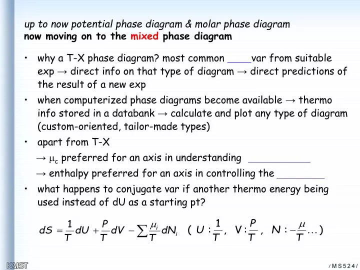
up to now potential phase diagram & molar phase diagram now moving on to the mixed phase diagram

1. up to now potential phase diagram & molar phase diagram now moving on to the mixed phase diagram • why a T-X phase diagram? most common var from suitable exp → direct info on that type of diagram → direct predictions of the result of a new exp • when computerized phase diagrams become available → thermo info stored in a databank → calculate and plot any type of diagram (custom-oriented, tailor-made types) • apart from T-X → mc preferred for an axis in understanding → enthalpy preferred for an axis in controlling the • what happens to conjugate var if another thermo energy being used instead of dU as a starting pt?

2. from Chapter 4 of Saunders and Miodownik’s book, “CALPHAD” exp determination of thermo quantities → thermo measurements after Kubaschewski (1993) at Aachen ① methods - powerful for establishing integral and partial enthalpies - but limited use in partial Gibbs energy & activity or activity coefficient - measuring heat & during heating and cooling or from a rxn - its reliability governed by heat conduction, heat capacity & heat transfer efficiency isothermal : Ts(surr) = Tc(calorimeter), const T adiabatic : Ts = Tc, T not const, determining heat capacity heat-flow : Ts - Tc = constant isoperibol : const Ts, measuring Tc i) measurement of H & heat capacity - H  measuring HT - HRT vs T - heating the sample to high T and dropping it into a calor at low T - measuring heat evolved, not directly Cv - problems occur if Cv of calorimeter > Cv of the sample ii) measurement of enthalpy of transformation - DSC, DTA tech (ΔHtr can also be obtained from the method i)

3. ② 기상평형법 (gas phase equil tech) - activity, ai = pi/pi° → Gi & μi - how to measure , pi, correctly ③ (기전력) measurements - in electrochem cells  EMF generated  Gi, mi - ∆Gi= -nEF = RTln ai - ∆S & ∆H readily calculated from the above eq - providing good accuracy for ai & gi(act coeff) - H & S being associated with much higher errors

4. exp determination of phase diagrams ① non-isothermal tech - where a sample isorthrough a transf and some properties of the alloy changes as a consequence - inherently non-equil in nature - dealing with the of transf rather than the transf itself i) thermal analysis tech: typical simple cooling curve method by Haycock and Neville (1890, 1897) the curve of vs time preferred to T vs time more refined DSC or DTA methods be aware of or solid state diffusion in heating be aware of in cooling

5. Fig. 4.3 Cooling curve to determine liquidus point. Fig. 4.4 Liquidus points for Cu-Sn determined by Hycock and Neville (1890,1897). Fig. 4.5 Experimentally measured liquidus(Ο) and solidus (□) points measured by using DTA by Evans and Prince (1978) for In-Pb. (●) refers to the ‘near-equilibrium’ solidus found after employing re-heating/cycling method.

6. Fig. 4 DSC thermogram of solders taken at heating and cooling rates of 5°C/min. TS (solidus temp., set temp.) and TL(liquidus temp.) are recorded in the graph. (a) Sn-4Bi-2In-9Zn in heating. (b) 4Bi-2In-9Zn in cooling. (c) Sn-1Bi-5In-9Zn in heating, and (d) Sn-1Bi-5In-9Zn in cooling. Fig. 3.14 SiO2-Al2O3 system with sketches of representative DTA from cooling the specified composition.

7. Calculated isopleths of (a) Sn-Bi-2In-9Zn and (b) Sn-Bi-5In-9Zn alloys. Symbols of ∆, Ο, □ represent temperatures experimentally measured through DSC.

8. ii) chemical potential tech: activity of one or both of the comp being measured during a cooling or heating cycle and a series of characteristic breaks defining Fig. 4.6 EMF vs temperature measurements for Al-Sn alloys (Massart et al., 1965)

9. Fig. 4.7 Magnetic susceptibility () vs temperature measurements for a Fe-0.68at%Nb alloy (Ferrier et al. 1964). ●=heating, X=cooling Fig. 4.8 Plot of resistivity vs temperature for a Al-12.6at%Li alloy (Costas and Marshall, 1962). ⅲ) magnetic susceptibility measurement: an interesting tech for determining phase boundaries in systems ⅳ) resistivity method: a simple tech, the resistivity of an alloy during measured as a ft of T

10. Fig. 4.9 Expansion vs temperature plot for a (Ni79.9Al20.1)0.87Fe0.13 alloy showing ’/’+-phase boundary at 1159°C from Cahn et al. (1987). Fig. 4.10 ’/’+-phase boundary as a function of Fe constent, at a constant Ni/Al ratio=77.5/22.5 (from Cahn et al. 1987). ⅴ) dilatometric method: a sensitive method, in phase transf having different coeff of

11. ② isothermal tech (const T) inherently closer to → substantial periods to allow equil needed → how long is enough? → no easy ans → (as a first approx) (x : grain size) i) metallogrophy: OM, BS-SEM → phase boundary, identification & qualitative delineation of phases (heavy elements appearing light, light elements dark) Fig. 4.11 Equilibrium phase diagram for the Mo-Re system after Knapton (1958-59).

12. Fig. 4.12 Lattice parameter vs composition measurements for Hf(1-c)C (Rudy 1969). ii) XRD: used to support some other tech, identification of and a more exact determine of phase boundary using

13. iii) quantitative determination of phase : STEM, EDX & AP/FIM ⅳ) sampling/equilibration method: - in equil involving liq + sol → removal of some of the liq → defining liquidus comp - using the different density of liq and sol (gravity then sufficient for separation) ⅴ) diffusion couple: increased use of EPMA →

14. Fig. 4.13 Measured diffusion path between alloys, A and B, in the Ni-Al-Fe system at 1000°C (Cheng and Dayanada 1979). Fig. 4.14 Concentration profile in a diffusion couple from the Al-Nb-Ti system at 1200°C (Hellwig 1990).