Download
1 / 23
230 likes | 342 Views
Chapter 9: Rule Mining. 9.1 OLAP 9.2 Association Rules 9.3 Iceberg Queries. Monitoring & Administration. Metadata. Repository. OLAP. Servers. OLAP. Data Warehouse. External. Extract. sources. Transform. Query/Reporting. Load. Operational. Serve. DBS. Data Mining. Data sources.

E N D
Chapter 9: Rule Mining 9.1 OLAP 9.2 Association Rules 9.3 Iceberg Queries
Monitoring & Administration Metadata Repository OLAP Servers OLAP Data Warehouse External Extract sources Transform Query/Reporting Load Operational Serve DBS Data Mining Data sources Front-End Tools Data Marts • Mining business data for interesting facts and decision support • (CRM, cross-selling, fraud, trading/usage patterns and exceptions, etc.) • with data from different production sources integrated into data warehouse, • often with data subsets extracted and transformed into data cubes 9.1 OLAP: Online Analytical Processing
Typical OLAP (Decision Support) Queries • What were the sales volumes by region and product category • for the last year? • How did the share price of computer manufacturers • correlate with quarterly profits over the past 10 years? • Which orders should we fill to maximize revenues? • Will a 10% discount increase sales volume sufficiently? • Which products should we advertise to the various • categories of our customers? • Which of two new medications will result in the best outcome: • higher recovery rate & shorter hospital stay? • Which ads should be on our Web site to which category of users? • How should we personalize our Web site based on usage logs? • Which symptoms indicate which disease? • Which genes indicate high cancer risk?
Data Warehouse with Star Schema data often comes from different sources of different organizational units data cleaning is a major problem
7 1 2 4 5 6 3 • organize data (conceptually) into a multidimensional array • analysis operations (OLAP algebra, integrated into SQL): • roll-up/drill-down, slice&dice (sub-cubes), pivot (rotate), etc. Data Cube Example: sales volume as a function of product, time, geography Fact data: sales volume in $100 City City LA SF Dimensions: NY 117 Product, City, Date 10 Juice Attributes: Cola 50 Product (prodno, price, ...) Product Product Milk 20 Attribute Hierarchies and Lattices: Cream 12 Industry Country Year Toothpaste 15 10 Soap Category State Quarter Product City Month Week Date Date for high dimensionality: cube could be approximated by Bayesian net Date
9.2 Association Rules given: a set of items I = {x1, ..., xm} a set (bag) D={t1, ..., tn} of item sets (transactions) ti = {xi1, ..., xik} I • wanted: • rules of the form X Y with X I and Y I such that • X is sufficiently often a subset of the item sets ti and • when X ti then most frequently Y ti holds, too. support (X Y)= P[XY] = relative frequency of item sets that contain X and Y confidence (X Y)= P[Y|X] = relative frequency of item sets that contain Y provided they contain X support is usually chosen in the range of 0.1 to 1 percent, confidence (aka. strength) in the range of 90 percent or higher
Association Rules: Example Market basket data („sales transactions“): t1 = {Bread, Coffee, Wine} t2 = {Coffee, Milk} t3 = {Coffee, Jelly} t4 = {Bread, Coffee, Milk} t5 = {Bread, Jelly} t6 = {Coffee, Jelly} t7 = {Bread, Jelly} t8 = {Bread, Coffee, Jelly, Wine} t9 = {Bread, Coffee, Jelly} support (Bread Jelly) = 4/9 support (Coffee Milk) = 2/9 support (Bread, Coffee Jelly) = 2/9 confidence (Bread Jelly) = 4/6 confidence (Coffee Milk) = 2/7 confidence (Bread, Coffee Jelly) = 2/4
Apriori Algorithm: Idea and Outline • Idea and outline: • proceed in phases i=1, 2, ..., each making a single pass over D, • and generate rules X Y • with frequent item set X (sufficient support) and |X|=i in phase i; • use phase i-1 results to limit work in phase i: • antimonotonicity property (downward closedness): • for i-item-set X to be frequent, • each subset X‘ X with |X‘|=i-1 must be frequent, too • generate rules from frequent item sets; • test confidence of rules in final pass over D Worst-case time complexity is exponential in I and linear in D*I, but usual behavior is linear in D (detailed average-case analysis is very difficult)
Apriori Algorithm: Pseudocode procedure apriori (D, min-support): L1 = frequent 1-itemsets(D); for (k=2; Lk-1 ; k++) { Ck = apriori-gen (Lk-1, min-support); for each t D { // linear scan of D Ct = subsets of t that are in Ck; for each candidate c Ct {c.count++}; }; Lk = {c Ck | c.count min-support}; }; return L = k Lk; // returns all frequent item sets procedure apriori-gen (Lk-1, min-support): Ck = : for each itemset x1 Lk-1 { for each itemset x2 Lk-1 { if x1 and x2 have k-2 items in common and differ in 1 item // join { x = x1 x2; if there is a subset s x with s Lk-1 {disregard x;} // infreq. subset else add x to Ck; }; }; }; return Ck
Algorithmic Extensions and Improvements • hash-based counting (computed during very first pass): • map k-itemset candidates (e.g. for k=2) into hash table and • maintain one count per cell; drop candidates with low count early • remove transactions that don‘t contain frequent k-itemset • for phases k+1, ... • partition transactions D: • an itemset is frequent only if it is frequent in at least one partition • exploit parallelism for scanning D • randomized (approximative) algorithms: • find all frequent itemsets with high probability (using hashing etc.) • sampling on a randomly chosen subset of D • ... • mostly concerned about reducing disk I/O cost • (for TByte databases of large wholesalers or phone companies)
quantified rules: consider quantitative attributes of item in transactions • (e.g. wine between $20 and $50 cigars, or • age between 30 and 50 married, etc.) • constrained rules: consider constraints other than count thresholds, • e.g. count itemsets only if average or variance of price exceeds ... • generalized aggregation rules: rules referring to aggr. functions other • than count, e.g., sum(X.price) avg(Y.age) • multilevel association rules: considering item classes • (e.g. chips, peanuts, bretzels, etc. belonging to class snacks) • sequential patterns • (e.g. an itemset is a customer who purchases books in some order, • or a tourist visiting cities and places) • from strong rules to interesting rules: • consider also lift (aka. interest) of rule X Y: P[XY] / P[X]P[Y] • correlation rules • causal rules Extensions and Generalizations of Assocation Rules
example for strong, but misleading association rule: tea coffee with confidence 80% and support 20% but support of coffee alone is 90%, and of tea alone it is 25% tea and coffee have negative correlation ! Correlation Rules consider contingency table (assume n=100 transactions): T T C 20 70 90 {T, C} is a frequent and correlated item set C 5 5 10 25 75 correlation rules are monotone (upward closed): if the set X is correlated then every superset X‘ X is correlated, too.
example for strong, but misleading association rule: tea coffee with confidence 80% and support 20% but support of coffee alone is 90%, and of tea alone it is 25% tea and coffee have negative correlation ! Correlation Rules consider contingency table (assume 100 transactions): T T • E[C]=0.9 • E[T]=0.25 • E[(T-E[T])2]=1/4 * 9/16 +3/4 * 1/16= 3/16=Var(T) • E[(C-E[C])2]=9/10 * 1/100 +1/10 * 1/100 = 9/100=Var(C) • E[(T-E[T])(C-E[C])]= • 2/10 * 3/4 * 1/10 • 7/10 * 1/4 * 1/10 • 5/100 * 3/4 * 9/10 • + 5/100 * 1/4 * 9/10 = • 60/4000 – 70/4000 – 135/4000 + 45/4000 = - 1/40 = Cov(C,T) • (C,T) = - 1/40 * 4/sqrt(3) * 10/3 -1/(3*sqrt(3)) - 0.2 C 20 70 90 C 5 5 10 25 75
procedure corrset (D, min-support, support-fraction, significance-level): for each x I compute count O(x); initialize candidates := ; significant := ; for each item pair x, y I with O(x) > min-support and O(y) > min-support { add (x,y) to candidates; }; while (candidates ) { notsignificant := ; for each itemset X candidates { construct contingency table T; if (percentage of cells in T with count > min-support is at least support-fraction) { // otherwise too few data for chi-square if (chi-square value for T significance-level) {add X to significant} else {add X to notsignificant}; }; //if }; //for candidates := itemsets with cardinality k such that every subset of cardinality k-1 is in notsignificant; // only interested in correlated itemsets of min. cardinality }; //while return significant Correlated Item Set Algorithm
Queries of the form: Select A1, ..., Ak, aggr(Arest) From R Group By A1, ..., Ak Having aggr(Arest) >= threshold 9.3 Iceberg Queries with some aggregation function aggr (often count(*)); A1, ..., Ak are called targets, (A1, ..., Ak) with an aggr value above the threshold is called a frequent target Baseline algorithms: 1) scan R and maintain aggr field (e.g. counter) for each (A1, ..., Ak) or 2) sort R, then scan R and compute aggr values but: 1) may not be able to fit all (A1, ..., Ak) aggr fields in memory 2) has to scan huge disk-resident table multiple times Iceberg queries are very useful as an efficient building block in algorithms for rule generation, interesting-fact or outlier detection (on market baskets, Web logs, time series, sensor streams, etc.)
Examples for Iceberg Queries Market basket rules: Select Part1, Part2, Count(*) From All-Coselling-Part-Pairs Group By Part1, Part2 Having Count(*) >= 1000 Select Part, Region, Sum(Quantity * Price) From OrderLineItems Group By Part, Region Having Sum(Quantity*Price) >= 100 000 Frequent words (stopwords) or frequent word pairs in docs Overlap in docs for (mirrored or pirate) copy detection: Select D1.Doc, D2.Doc, Count(D1.Chunk) From DocSignatures D1, DocSignatures D2 Where D1.Chunk = D2.Chunk And D1.Doc != D2.Doc Group By D1.Doc, D2.Doc Having Count(D1.Chunk) >= 30 table R should avoid materialization of all (doc chunk) pairs
V: set of targets, |V|=n, |R|=N, V[r]: rth most frequent target H: heavy targets with freq. threshold t, |H|=max{r | V[r] has freq. t} L = V-H: light targets, F: potentially heavy targets Acceleration Techniques Determine F by sampling scan s random tuples of R and compute counts for each x V; if freq(x) t * s/N then add x to F or by „coarse“ (probabilistic) counting scan R, hash each x V into memory-resident table A[1..m], m<n; scan R, if A[h(x)] t then add x to F Remove false positives from F (i.e., x F with x L) by another scan that computes exact counts only for F Compensate for false negatives (i.e., x F with x H) e.g. by removing all H‘ H from R and doing an exact count (assuming that some H‘ H is known, e.g. „superheavy“ targets)
Defer-Count Algorithm Key problem to be tackled: coarse-counting buckets may become heavy by many light targets or by few heavy targets or combinations 1) Compute small sample of s tuples from R; Select f potentially heavy targets from sample and add them to F; 2) Perform coarse counting on R, ignoring all targets from F (thus reducing the probability of false positives); Scan R, and add targets with high coarse counts to F; 3) Remove false positives by scanning R and doing exact counts Problems: difficult to choose values for tuning parameters s and f phase 2 divides memory between initial F and hash table for counters
Multi-Scan Defer-Count Algorithm 1) Compute small sample of s tuples from R; Select f potentially heavy targets from sample and add them to F; 2) for i=1 to k with independent hash functions h1, ..., hk do perform coarse counting on R using hi, ignoring targets from F; construct bitmap Bi with Bi[j]=1 if j-th bucket is heavy 3) scan R and add x to F if Bi[hi(x)]=1 for all i=1, ..., k; 4) remove false positives by scanning R and doing exact counts + further optimizations and combinations with other techniques
Multi-Level Algorithm 1) Compute small sample of s tuples from R; Select f potentially heavy targets from sample and add them to F; 2) Initialize hash table A: mark all h(x) with xF as potentially heavy and allocate m‘ auxiliary buckets for each such h(x); set all entries of A to zero 3) Perform coarse counting on R: if h(x) is not marked then increment h(x) counter else increment counter of h‘(x) auxiliary bucket using a second hash function h‘; scan R, and add targets with high coarse counts to F; 4) Remove false positives by scanning R and doing exact counts Problem: how to divide memory between A and the auxiliary buckets
R = {1, 2, 3, 4, 1, 1, 2, 4, 1, 1, 2, 4, 1, 1, 2, 4, 1, 1, 2, 4}, N=20 threshold T=8 H={1} hash function h1: dom(R) {0,1}, h1(1)=h1(3)=0, h1(2)= h1(4)=1, hash function h2: dom(R) {0,1}, h2(1)=h2(4)=0, h2(2)=h2(3)=1, Iceberg Query Algorithms: Example Defer-Count: s=5 F={1} using h1: cnt(0)=1, cnt(1)=10 bitmap 01, re-scan F={1, 2, 4} final scan with exact counting H={1} Multi-scan Defer-Count: s=5 F={1} using h1: cnt(0)=1, cnt(1)=10 using h2: cnt(0)=5, cnt(1)=6 re-scan F={1} final scan with exact counting H={1}
J. Han, M. Kamber, Chapter 6: Mining Association Rules • D. Hand, H. Mannila, P. Smyth: Principles of Data Mining, MIT Press, • 2001, Chapter 13: Finding Patterns and Rules • M.H. Dunham, Data Mining, Prentice Hall, 2003, Ch. 6: Association Rules • M. Ester, J. Sander, Knowledge Discovery in Databases, Springer, 2000, • Kapitel 5: Assoziationsregeln, Kapitel 6: Generalisierung • M. Fang, N. Shivakumar, H. Garcia-Molina, R. Motwani, J.D. Ullman: • Computing Iceberg Queries Efficiently, VLDB 1998 • S. Brin, R. Motwani, C. Silverstein: Beyond Market Baskets: • Generalizing Association Rules to Correlations, SIGMOD 1997 • C. Silverstein, S. Brin, R. Motwani, J.D. Ullman: Scalable Techniques for • Mining Causal Structures, Data Mining and Knowledge Discovery 4(2), 2000 • R.J. Bayardo: Efficiently Mining Long Patterns from Databases, SIGMOD 1998 • D. Margaritis, C. Faloutsos, S. Thrun: NetCube: A Scalable Tool • for Fast Data Mining and Compression, VLDB 2001 • R. Agrawal, T. Imielinski, A. Swami: Mining Association Rules • Between Sets of Items in Large Databases, SIGMOD 1993 • T. Imielinski, Data Mining, Tutorial, EDBT Summer School, 2002, • http://www-lsr.imag.fr/EDBT2002/Other/edbt2002PDF/ • EDBT2002School-Imielinski.pdf • R. Agrawal, R. Srikant, Whither Data Mining?, • http://www.cs.toronto.edu/vldb04/Agrawal-Srikant.pdf Additional Literature for Chapter 9