Download
1 / 23
230 likes | 358 Views
Intermolecular Forces and Liquids and Solids. Chapter 11. Fig 11.19 Heating curve for water Indicates changes when 1.00 mol H 2 O is heated from 25°C to 125°C at constant P. Sample Exercise 11.4 Calculating Δ H for Temperature and Phase Changes.

E N D
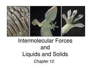
Intermolecular Forces and Liquids and Solids Chapter 11
Fig 11.19 Heating curve for water Indicates changes when 1.00 mol H2O is heated from 25°C to 125°C at constant P
Sample Exercise 11.4 Calculating ΔH for Temperature and Phase Changes Calculate the enthalpy change upon converting 1.00 mol of ice at –25 oC to water vapor (steam) at 125 oC under a constant pressure of 1 atm. The specific heats of ice, water, and steam are 2.03 J/g-K, 4.18 J/g-K, and 1.84 J/g-K, respectively. For H2O, ΔHfus = 6.01 kJ/mol and ΔHvap = 40.67 kJ/mol.
“Dynamic Equilibrium” Rate of evaporation Rate of condensation = Vapor pressure - the pressure of a vapor measured when a dynamic equilibrium exists between evaporation and condensation Fig 11.22 Equilibrium vapor pressure over a liquid
Fig 11.23 Effect of temperature on the distribution of kinetic energies in a liquid
Vapor Pressure and Boiling Point Fig 11.24 • Boiling point ≡ temperature at which its vapor pressure equals atmospheric pressure • Normal boiling point ≡ temperature at which its vapor pressure is 760 torr
Clausius-Clapeyron Equation ln P = − DHvap + C RT Molar heat of vaporization (DHvap) ≡ the energy required to vaporize 1.00 mole of a liquid P = (equilibrium) vapor pressure T = temperature (K) R = gas constant (8.314 J/K•mol) m = −DHvap/R ln P 1/T
lnP1 = − lnP2 = − DHvap DHvap + C + C RT1 RT2 Clausius-Clapeyron Equation P = (equilibrium) vapor pressure m = DHvap/R T = temperature (K) ln P R = gas constant (8.314 J/K∙mol) 1/T
Phase Diagrams • Display the state of a substance at various pressures and temperatures and the places where equilibria exist between phases Fig 11.26 Phase diagram for a three-phase system
Phase Diagram of Water Fig 11.27 (a) • Note the negative slope of the solid-liquid equilibrium line • Implies that ice melts at a lower temperature when pressure is increased • T = triple point, where solid, • liquid, and vapor coexist in • equilibrium
Phase Diagram of Carbon Dioxide Fig 11.27 (b) • CO2 sublimes at normal pressures • CO2 cannot exist in the liquid state at pressures below 5.11 atm; • CO2 becomes a supercritical • fluid anywhere above Point C
Supercritical CO2 Fig 11.20 The low critical temperature and critical pressure for CO2 make supercritical CO2 a good solvent for extracting nonpolar substances (like caffeine)
Diagram of a supercritical fluid extraction process Fig 11.21
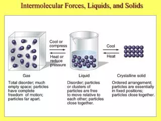
Structures of Solids • Crystalline-particles are in highly ordered arrangement • Amorphous– no particular order in the arrangement of particles
Crystalline Solids • Because of the order in a crystal, we can focus on the repeating pattern of arrangement called the unit cell
Fig 11.35 Two ways of defining the unit cell of NaCl Cl− at lattice points or Na+ at lattice points • Both are acceptable choices
Attractions in Ionic Crystals In ionic crystals, ions pack themselves so as to maximize the attractions and minimize repulsions between the ions. Hexagonal close-packed Cubic close-packed
Covalent-Network andMolecular Solids Fig 11.41 sp2 hybridized sp3 hybridized diamond graphite • Diamonds tend to be hard and have high melting points • Graphite is slippery due to weak dispersion forces between sheets • Tend to be softer and have lower melting points
Fig 11.43 The buckminsterfullerene molecule, C60 The 60 carbon atoms sit at the vertices of a truncated icosahedron—the same geometry as a soccer ball
Metallic Solids Fig 11.45 • Metals not covalently bonded • Attractions between atoms are too strong to be van der Waals forces • In metals valence electrons are delocalized throughout the solid • “Electron-sea model”
Table 11.7 Types of Bonding in Crystalline Solids