Download
1 / 43
740 likes | 1.45k Views
INVENTORY ANALYSIS. MM – OM – Session 6 Henry Yuliando. ...Cases. Three largest booksellers in US: Borders Group, Barnes&Noble, and Amazon. Borders Group has 174 days of inventory in its network; Barnes&Noble 129 days in 2006.

E N D
INVENTORY ANALYSIS MM – OM – Session 6 Henry Yuliando
...Cases • Three largest booksellers in US: Borders Group, Barnes&Noble, and Amazon. • Borders Group has 174 days of inventory in its network; Barnes&Noble 129 days in 2006. • From a macroeconomic perspective, inventort-related cost accounted approx. 2.5% of the GDP of US in 2005.
Different Views of INVENTORY Demand Type Independent Dependent Annual $ Volume ABC analysis Types Cycle Pipeline Safety Stock Anticipation Process stage Raw material Work in Proces Finished goods Other: Maintenance/Repair Operating Supplies
Inventory Classification of an Automobile Firm Engine Plant Assembly Plant Dealership Autombile firm
Inventory Benefits • Economies of scale • Procuring inputs involves a fixed order cost – as a fraction of total cost, this cost is independent of order size. • In producing outputs, starting process may involve a fixed setup cost – the time and materials required to set up a process. (e.g. Clean equipment and change tools) • The order or production in response to the economies of scale effect is referred as a batch. • Depending on the type of activity being performed: production batch (lot); transfer batch; procurement batch (order). • Cycle inventory is the average inventory arising due to a batch activity.
Inventory Benefits • Production and Capacity Smoothing. When demand fluctuates seasonally, it is more economical to maintain a constant processing rate and build inventories in periods of low demand and deplete them when demand is high (level-production strategy). • Stockout Protection. Inventories maintained to insulate the process unexpected supply disruptions or surges in demand are called safety inventory or safety stock. • Price Speculation.
Inventory Costs Inventory holding cost has two components : • Physical holding cost, refers to the cost of storing inventory. (e.g. Insurance, security, warehouse rental, lighting, and heating/cooling, etc). This cost is usually expressed as a fraction h of the variable cost C, thus physical holding cost = hC. • Opportunity cost, refers to the forgone return of the funds invested in inventory which could have been invested in alternate projects. Expressed as rC, where ris the firm rate of return and C is the variable cost. Then, Total unit inventory holding cost (H) = (h + r) C
Inventory Cost,..example • Centura Health is a nine-hospital integrated delivery network based in Denver, US. Presently, each hospital orders its own supplies and manages the inventory. • A common item used is a sterile Intravenous (IV) Starter Kit. • The weekly demand for this kit is 600 units (weekly R), which a unit cost of $3. • Centura has estimated that the physical holding cost (operating and storage cost) of one unit medical supply is about 5% per year (h). • The hospital network’s annual cost of capital is 25% (or $0.25 = r). • Each hospital incurs a fixed order cost of $130 whenever places an order. • The supplier takes one week to deliver the order. • Presently, each hospital places 6000 units per order. • Centura has recently been concerned about the level of inventories held of the hospitals and is exploring strategies to reduce them.
Inventory Cost • Consider Centura Health case, the annual physical holding cost H = (h + r) C = (0.05 + 0.25) 3 = $0.90 • Then, the total inventory holding cost per unit of time is H x I.
Inventory Dynamics of Batch Purchasing • The rest of this lesson is focused on the effect of economies of scale. • For an instance, an important managerial question of Centura Health: • How muchto purchase at a time? • Whento purchase a new batch of IV Starter Kits? • Consider following inventory dynamics of process view of Centura Health Input (IV starter kits) Output (orders) Order fullfilment (in-process inventory) Inputs inventory
Inventory Dynamics of Batch Purchasing • Recall case of Centura Health, it processes a demand of 600 units of the IV starter kit each week and places and order of 6000 kits at a time. • The hospital must then be ordering once every 10 weeks. • Average IV starter kit inventory will be Icycle = 6000/2 = 3000 units, and a typical kit spend and average of five week in storage. • Consider a cost effective to order (or produce) in batches, such as a case ATM, training, shuttle bus service, trash collection, etc.
Economies of Scale and Optimal Cycle Inventory • Two causes of scale economies: • Economies arising from a fixed-cost component of costs in either procurement (e.g. order cost), production (e.g. setup cost), or transportation. • Economies arising from price discount offered by suppliers.
Economies of Scale and Optimal Cycle Inventory Fixed Cost of Procurement: Economic Order Quantity • Process manager can control inflow into the buffer. • The total annual fixed order cost = S X R/Q • Total holding cost per year : H x Icycle = H x (Q/2) • Total annual cost of material procured = unit cost x ouflow rate = C x R • Thus the total annual cost, TC, is given by : • Recall Centura Health case, fixed cost per order of IV starter kit = $130. The unit cost C = $3, and weekly outflow rate of 600 or equal to an annual outflow rate = 31,200 per year (assuming 52 weeks).
Economies of Scale and Optimal Cycle Inventory Fixed Cost of Procurement: Economic Order Quantity • As Centura holding cost per year H = $0.90, and Q = 6000 units in each order, the component of the total annual cost: Total annual fixed order cost = S x R/Q = 130 x 31,200/6000 = $676 Total annual holding cost = H x (Q/2) = 0.90 x 3000 = $2700 Total annual cost of materials = C x R = 3 x 31,200 = $93,600 Thus, total annual cost = $96,976
I(t) Ip + Q -R Q Q Q Ip tz 2tz 0 t
Economies of Scale and Optimal Cycle Inventory Order Q = 3000 gives the total minimum cost
Costs Total cost TC* Inventory holding cost Variable (material) cost Fixed order cost Q* = EOQ
Economies of Scale and Optimal Cycle Inventory Fixed Cost of Procurement: Economic Order Quantity • Based on the above graph, The economic order quantity (EOQ) is the optimal order quantity that minimizes total fixed and variable cost of a batch order (Q*). • Based on EOQ: Total annual fixed costs per order = total annual holding costs, thus S x R/Q* = H x (Q*/2), and the minimum in actual total cost, TC* = 2 S R H + CR • Using example of Centura Health hospitals network:
Economies of Scale and Optimal Cycle Inventory Fixed Order Cost Reduction • The optimal order size increase if the fixed order cost increases. • Fixed cost in procurement usually include administrative costs of creating a purchase order, activities or receiving the order, so on. • Technology can be used significantly to reduce such costs, for example Electronic Data Interchange (EDI) success story of Wal Mart.
Economies of Scale and Optimal Cycle Inventory Inventory versus Sales Growth • Te EOQ formula is relevant to proof that a doubling of a company’s annual sales does not require a doubling of invetory cycle. Centralization and Economies of Scale • The idea of inventory centralization (logistics in practices) ireferred to the fact that the optimal batch Q* is proportional to the square root of the outflow rate R. • Consider Centura Health case, it could centralize purchasing of all supplies and perhaps store these in a central warehouse. Assuming that the cost parameters unchanged, it could expect that for total outflow rate that is nine hospitals, the average inventory would be only three times (equal to 9)
Economies of Scale and Optimal Cycle Inventory Centralization and Economies of Scale • Consider Centura Health case, S = $130; and H = $0.90, weekly outflow rate (R)= 600 for each hospital. The EOQ (Q*) = 3,002 units; Icycle = 1,502 units. Total annual order and holding cost = $2,702. • If 9 hospital assummed to be identical: The total cycle inventory = 9 x 1,501 = 13,509 units The total annual and holding costs = 9 x $2,702 = $24,318 Annual outflow rate of 9 hospitals = 9 x 31,200/year = 280,800 units/year Here, the new EOQ = The inventory cycle = 9,006/2 = 4,503; with the total annual order and holding costs = which is 67% lower than for the decentralized operation.
Effect of Lead Times on Ordering Decision • Lead time(L) is the time lag between the arrival of the replenishment and the time the order was placed. • Reorder point (ROP) is the availble inventory at the time of placing an order. ROP = L x R • Ex., recall Centura Health case, the replenishment lead time for ordering IV starter kits is L = 1 week. Then ROP = L x R = 1 week x 600 units/week = 600.
Effect of Lead Times on Ordering Decision Ordering Decisions and The Reorder Point, case L < Q/R
EOQ without the instantaneous receipt assumption • This model is applicable when inventory continuously flows or builds up over a period of time after an order has been placed or when units are produced and sold simultaneously. (called production run model) There is no production during this part of the inventory cycle Inventory level Part of inventory cycle during which production is taking place Maximum inventory Time t
Annual cost for production run model • Q = number of pieces per order, or production run • Cs = setup cost • Ch = holding cost per unit per year • p = daily production rate • R = annual outflow (annual demand rate) • d = daily demand rate • t = length of production run in days • Total produced = Q = pt or t =Q/p • The maximum inventory level = pt – rt = Q(1-r/p) • Average inventory = Q/2(1-r/p) • Annual holding cost = Q/2(1-r/p)Ch • Annual setup cost = (R/Q)Cs • The optimal production quantity is
Single-item static model with price breaks Quantity Discount Model • The total cost = material cost + ordering cost + carrying cost Total cost = DC + (D/Q)Co + (D/Q)Ch where D = annual demand in units Co = ordering cost of each order C = cost per unit Ch = holding or carrying cost per unit per year Ch = hC (h = percentage of the unit cost C)
Total cost $ TC curve for Discount 1 TC curve for Discount 3 • For each discount price ( C ), EOQ = • If EOQ < minimumfor discount, adjust the quantity to Q = minimum for discount. • For each EOQ or adjusted Q, total cost = DC + (D/Q)Co + (D/Q)Ch • Choose the lowest cost quantity. TC curve for Discount 2 EOQ for Discount 2 1000 2000 Order quantity
Price Discounts: Forward Buying • For a trade promotion, it is often that a supplier give a short-term discount policy. • The supplier offers incentives in the form of one-time opportunities to sell materials at reduced unit costs or perhaps notifies the buyer of an upcoming price increase and offers one last chance to order at the lower price.
Consider that instead of a normal price of $C per unit, a supplier offers a one-time discount of $d per unit. Then for a certain period the price is $(C-d)/unit • After which the regular price will resume, the buyer must decide the quantity Qf to order at the discounted price. • The optimal forward-buying quantity is computed as follows:
… • Example: Kmart-retail store to order toothpaste Colgate S = order cost = $100 R= unit demand per year = 120,000 C = unit price = $3 h = unit annual holding cost = 0.2 d = discounted amount of price (ex : for one time discount 5%, at regular price C = $3 / unit, d = 0.05x$3 = $0.15) H = unit annual holding cost = $0.60 Q* = regular optimum order quantity
SAFETY INVENTORY and SERVICE LEVEL Service Level Measures: • Cycle service level, refers to either the probability that there will be no stockout within an order cycle, or, equivalently, the proportion of order cycles without a stockout, where an order cycle is the time between two consecutive replenishment orders. • Fill rate, is the fraction of total demand satisfied from inventory on hand.
SAFETY INVENTORY and SERVICE LEVEL Service Level Measures: • For example: a process manager observes that within 100 order cycles, stockouts occurs in 20. Cycle service level is then 80/100 = 80% • Now suppose that total demand during 100 cycles was 15,000 units and the total number of units short in the 20 cycles with stockouts was 1,500 units. The fill rate, therefore, 13,500/15,000 = 0.9 or 90%.
SAFETY INVENTORY and SERVICE LEVEL Continuous Review, Reorder Point System • Lead Time Demand (LTD), isthe total flow-unit requirement during replenishment lead time (L). • In general, if either flow rate R or lead time L is uncertain, the LTD will also be uncertain. • To reduce stockout risk, we may decide to order earlier by setting the reorder point larger than LTD. • The excess amount is safety inventory (Isafety) Isafety = ROP – LTD or ROP = LTD + Isafety
SAFETY INVENTORY and SERVICE LEVEL Service Level Given Safety Inventory • Service level (SL) is the probability that the actual LTD will not exceed ROP, or SL = Prob(LTD ROP) • To compute this probability, it is necessary to know the probability distribution of the random variable LTD (assumed normally distributed) with mean LTD and standard deviation LTD.
SAFETY INVENTORY and SERVICE LEVEL Service Level Given Safety Inventory
SAFETY INVENTORY and SERVICE LEVEL • Correspoding to the z value: SL = Prob(LTD ROP) = Prob (Z ≤ z) Isafety = z x LTDor SL = NORMDIST (ROP, LTD, LTD,True) • Example: GE Lightings has the average LTD = 20,000 units with LTD = 5,000. The warehouse currently orders a 14-day supply of lamps at ROP = 24,000 units. Determine SL? Isafety = ROP – LTD = 4,000 SL = Prob (Z ≤ 0.8) = 0.7881 or SL = NORMDIST(24,000,20,000,5,000,True) = 0.7881
SAFETY INVENTORY and SERVICE LEVEL • To summarize, in 78.81% of the order cycles, the warehouse will not have a stockout. • Recall that Q = 28,000 units, thus: Icycle = 28,000/2 = 14,000 Isafety= 4,000 Inventory total = 18,000 units H = $20 x 18,000 = $360,000/year T = I/R = 18,000/2,000 = 9 days
SAFETY INVENTORY and SERVICE LEVEL Safety InventoryGiven Service Level • Service level (SL) is known and need to determine safety inventory and ROP. SL = Prob (Z ≤ z) or z = NORMSINV (SL) Isafety = z x LTD and ROP = LTD + Isafety ROP = NORMINV (SL, LTD, LTD) • Example: Reverse case of GE Lightings, with know SL = 78.81, obtains Isafety = 4,000 and ROP = 24,000.
SAFETY INVENTORY and SERVICE LEVEL Safety InventoryGiven Service Level
The effect of Everyday Low Pricing • Order incerases designed to take an advantage of short-term discount. • A policy of everyday low pricing (EDLP) – a pricing policy whereby retailers charge constant, with no temporary discount. • The same argument can be used upstream in the supply chain.
Levers for Managing Inventory • Theoretical inventory: reducing critical activity times; eliminating non-value-adding activities; moving work from critical to non-critical activities; redesigning the process to replace sequential with parallel processing. • Cycle inventory: reduce fixed order (setup) cost by simplifying the order process with the use of information technology; negotiating everyday low prices with suppliers. • Seasonal inventory: using pricing and incentive tactics to promote stable demand patterns. • Safety inventory: ensuring reliable suppliers and stable demand patterns (discussed further in next session). • Speculative inventory: reduce the total cost of purchasing materials; increases profits by taking advantage of uncertain fluctuations in a product’s price.