Download
1 / 62
620 likes | 635 Views
Delve into the historical evolution of cosmic models from Friedmann to Lemaître, understanding cosmological parameters, consequences of universe geometry, and the dynamics of an expanding universe. Explore key concepts such as dark energy, curvature of space, and the implications of Einstein's theories on the expanding universe, all discussed in this informative astronomy seminar.

E N D
Early models of an expanding Universe Paramita Barai Astr 8900 : Astronomy Seminar 5th Nov, 2003
Contents • Introduction • Discuss papers : • 1922 : Friedmann • 1927 : Lemaître • 1932 : Einstein & De Sitter • Present cosmological picture • Some results • SN project, WMAP, SDSS
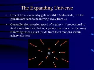
Cosmological foundations • Cosmological principle • Universe is Homogeneous & Isotropic on large scales (> 100Mpc) • Universe (space itself) expanding, dD/dt ~ D (Hubble Law) • Universe expanded from a very dense, hot initial state (Big Bang) • Expansion of universe – mass & energy content – explained by laws of GTR Dynamics of universe • Structure formation in small scales (<10-100 Mpc) by gravitational self organization • WHAT IS THE GEOMETRY OF OUR UNIVERSE, & IT’S CONSEQUENCES ??
Cosmological parameters • R – Scale factor of Universe • Critical density , C – density to make universe flat (it just stops expanding) • Density parameter, = / C • H = Hubble constant = v / r • = Cosmological Constant (still speculative!!) • Dark Energy • Repulsive force, opposing gravity
Curvature of space • Positive curvature – Closed – contract in future • > C • > 1 • Zero curvature – Flat – stop expansion in future & stationary • = C • = 1 • Negative curvature – Open – expand forever • < C • < 1
Timeline • 1905 – Einstein’s STR, 1915 – GTR • 1917 – Einstein & De Sitter static cosmological models with • 1922 – Friedmann • First non-static model • Universe contracts / expands (with ) • 1927 – Lemaître – expanding universe • 1930 – Hubble: expanding universe, Einstein drops (“biggest blunder”) • 1932 – Einstein & de Sitter • Expanding universe of zero curvature
Timeline – cont’d… • 1948 – Particle theory (QED) predicts non zero vacuum energy , but QED = 10120other • 1965 – CMBR • Early 1980’s: LUM << C Open universe • 1980’s – • Inflation theory Flat universe (TOT = 1) • Dark matter • 1990’s - LUM~ 0.02-0.04, DARK ~ 0.2-0.4, REST= ? • 1998 – Accelerating universe • Present model – universe very near to flat (with matter and vacuum energy)
Matter density = 0 Advantage : Explains naturally observed radial receding velocities of extra galactic objects From consequence of gravitational field Without assuming we are at special position Parameters c = velocity of light = Cosmological constant = Density of universe Two first models of universe:De Sitter
Non zero matter density Relation between density & radius of universe masses much greater than known in universe at that time Can’t explain receding motion of galaxies Advantage Explains existence of matter Parameters = Einstein constant = 1.8710-27 (cgs) Einstein universe
Curvature of space Aleksandr Friedman Zeitschrift fur Physik 10, 377-386, 1922
Summary • First non static model of universe • Work immediately not noticed, but found important later … • R independent of t : • Stationary worlds of Einstein & de Sitter • R depends on time only : • Monotonically expanding world • Periodically oscillating world • depending on chosen
Goal of the paper • Derive the worlds of Einstein & de Sitter from more general considerations
Assumptions of 1st class • Same as Einstein & de Sitter • Gravitational potentials obey Einstein field equations with cosmological term • Matter is at relative rest
Assumptions of 2nd class • Space curvature is constant wrt 3 space coordinates; but depends on time • Metric coefficients: g14, g24, g34 = 0, suitable choice of time coordinate
R(x4) = 0 M = M0 = constant Cylindrical world Einstein’s results M = (A0x4+B0) cos x1 Transform x4 De Sitter spherical world (M=cos x1) Solutions: Einstein & de Sitter worlds as special cases Stationary world
R(x4) 0 M = M(x4) But – suitable x4 – M = 1 Non stationary world
R ( > 0 ) Increases with t Initial value, R = R0 (>0) at t = t0 R = 0, at t = t t = Time since creation of world Monotonic world of first kind > 4c2/9A2
Time since creation of world, t R increases with t Initial R = x0 x0 & x0 are roots of equation: A-x+(x3/3c2) = 0 Monotonic world of second kind 0 < < 4c2/9A2
R – periodic function of t World Period = t Periodic World t if Small , approximate - < < 0
Possible universes of Friedmann • Monotonic worlds • > 4c2/9A2 • First kind • 0 < < 4c2/9A2 • Second kind • Periodic universe • - < < 0
Conclusions • Insufficient data to conclude which world our universe is … • Cosmological constant, is undetermined … • If = 0, M = 5 1021 M • Then, world period = 10 billion yrs • But this only illustrates calculation
A Homogeneous universe of Constant Mass & Increasing Radius accounting for the Radial Velocity of Extra – Galactic NebulaeAbbe Georges Lemaître • Annales de la Société scientifique de Bruxelles, A47, 49, 1927 • English translation in MNRAS, 91, 483-490, 1931
Summary • Dilemma between de Sitter & Einstein world models • Intermediate solution – advantages of both • R = R(t) • R(t) as t • Similar differential equation of R(t) as Friedmann
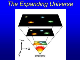
Summary cont’d.… • Accounted the following: • Conservation of energy • Matter density • Radiation pressure • Role in early stages of expansion of universe • First idea: • Recession velocities of galaxies are results of expansion of universe • Universe expanding from initial singularity, the ‘primeval atom’
Intermediate model • Solution intermediate to Einstein & De Sitter worlds • Both material content & explaining recession of galaxies • Look for Einstein universe • Radius varying with time arbitrarily
Universe ~ Sparsely dense gas Molecules ~ galaxies Uniformly distributed Density – uniform in space, time variable Ignore local condensation Internal stresses ~ Pressure p = (2/3) K.E. Negligible w.r.t energy of matter Radiation pressure of E.M. wave Weak Evenly distributed Keep p in general eqn For astronomical applications, p = 0 Assumptions of model
Field equations : conservation of energy • Einstein field equations • = Cosmological Constant (unknown) • = Einstein Constant • Total energy change + Work done by radiation pressure in the expanding universe = 0
= Total density = Matter density = - 3p Mass, M = V = constant = constant = integration constant Equations: Universe of constant mass
De Sitter world = 0 = 0 Einstein world = 0 R = constant Existing solutions
R0 = Initial radius of universe (from which expanding) R = Lemaître distance scale at time t RE = Einstein distance scale at t For = 0 & = 2R0 Lemaître solution
Cosmological Redshift • R1, R2 = Radius of Universe at times of emission & observation of light • Apparent Doppler effect • If nearby source, r = distance of source
Einstein radius of universe: by Hubble from mean density RE = 2.7 1010 pc If R0 from radial velocities of galaxies R from R3 = RE2 R0 From data R/R = 0.6810-27 cm-1 R0/R = 0.0465 R = 0.215RE = 6 109 pc R0 = 2.7 108 pc = 9 108 LY Values Calculated
Mass of universe – constant Radius of universe – increases from R0 (t = -) Galaxies recede as effect of expansion of universe Advantage of both Einstein & de Sitter solutions Conclusions
Expanding space Possible universe of Lemaître
100 Mt. Wilson telescope range: 5 107 pc = R / 200 Doppler effect – 3000 km/s Visible spectrum displaced to IR Why universe expands? Radiation pressure does work during expansion expansion set up by radiation itself Limitations & Further scopes
On the relation between Expansion & mean density of universeAlbert Einstein& Wilhelm de sitter(Proceedings of the National Academy of Sciences 18, 213 – 214, 1932)
Summary • After Hubble discovered expansion of universe: Einstein & de Sitter withdrew • Expanding universe – without space curvature • If matter = C= 3H2/(8G) • Euclidean geometry • Flat, infinite universe • Using H0 ~ 10 H0 today • G(optically visible galaxies) ~ C Flat space
Motivation • Observational data for curvature • Mean density • Expansion Universe – non static • Can’t find curvature sign or value • If can explain observation without curvature ??
to explain finite mean density in static universe Dynamic universe – without = 0 Line element: R = R(t) Neglect pressure (p) Field equation => 2 differential eqns Zero curvature
From observation H - coefficient of expansion - mean density From H = 500 km sec-1 Mpc-1 or, RB = 2 1027 cm Get RA = 1.63 1027 cm = 4 10-28 g cm-3 Coincide exactly with theoretical upper limit of density for Flat space Solutions
H – depends on measured redshifts Density – depends on assumed masses of galaxies & distance scale Extragalactic distances Uncertain H2 / or RA2/RB2 ~ /M = Side of a cube containing 1 galaxy = 106 LY M = average galaxy mass = 2 1011 M ~ close to Dr. Oort’s estimate of milky way mass Confidence limit of solution
- higher limit Correct magnitude order Possible to describe universe without curvature of 3-D space However, curvature is determinable More precise data Fix curvature sign Get curvature value Conclusions
Present status of cosmological model • Search for cosmological parameters determining dynamics of universe: • Hubble constant, H0 • TOT = M + + K • M = M/C • Matter (visible+dark) • = / 3H02 • Vacuum energy • K = -k / R02H02 • Curvature term • If flat k = 0
H0 Hubble key project WMAP H0 = (71 3) km/s/Mpc M Cluster velocity dispersion Weak gravitational lens effect visible ~ 0.02 – 0.04 dark ~ 0.25 M ~ 0.3 Current values
• Energy density of vacuum • Discrepancy of > 120 orders of magnitude with theory • ~ 0.7 • SN Type Ia • WMAP • Age of universe: • t0 = 13.7 G yr
SN Type Ia • Giant star accreting onto white dwarf • Standard candle • Compare observed luminosity with predicted • Far off SN fainter than expected • Expansion of Universe is accelerating
Microwave background fluctuations • Brightest microwave background fluctuations (spots): 1 deg across • Ground & balloon based experiments • Flat – 15 % accuracy • WMAP • Measures basic parameters of Big Bang theory & geometry of universe • Flat – 2 % accuracy