Handwriting: Registration and Differential Equations

1. Handwriting: Registration and Differential Equations

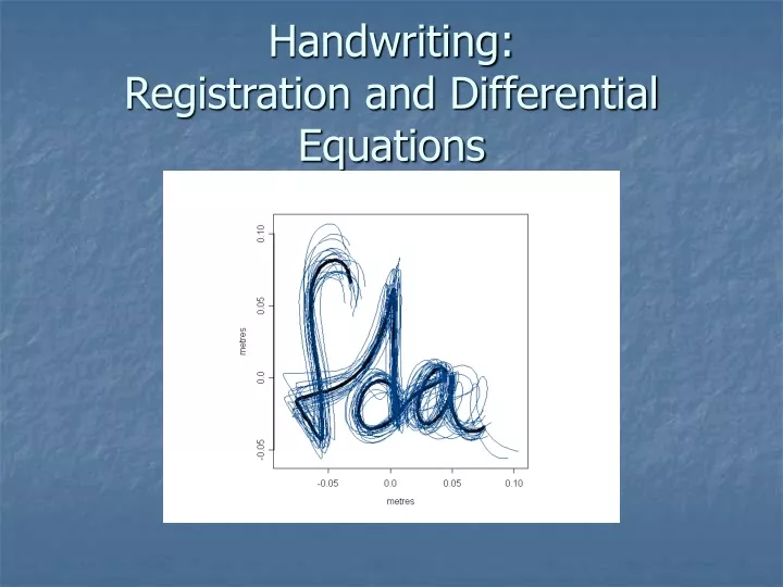
2. Printed the letters “fda” by hand 20 times. • Optotrak system recorded positions of pen, 200 times per second: • X (left to right) • Y (front to back) • Z (up and down, vertically) • There are different rates of printing, even for same person.

3. Why study time records of handwriting? • Fraud detection: handwriting is personal. • We usually only see static images – but what about our time-signature? Are our writing dynamics unique?

4. How can we prepare the data for analysis? • Problem: Timing of letters is different for each replication. • “Hand times” are different than “clock time.” • Amplitude differences: having to do with shape. • Phase differences: having to do with timing. • Both are important components of functional data. • How can we transform (warp) the clock time so that we’re left with only amplitude differences?

5. What does a warping function look like? • Target function is sin(4pit). • Individual function is running is fast: • So time-warping function is

6. What’s the process to align our data? • Idea: Rescale time with a warping function. • To do this, we need a “target” curve. • Can use a gold-standard curve, or use a mean curve, or iterate. • Time-warping function maps “clock time” to “hand time.” Continuous-Time Registration

7. First Problem: Need curves to fit in same interval. • Each curve i lasts over interval [0, Ti] • Want to rescale each curve to fit a target interval [0, T0] • Solution: Find a time-warping function hi(t) such that • hi(0) = 0 (starts at same time) • hi(T0) = Ti (ends at same time) • hi(t1) > hi(t2) iff t1 > t2 (events occur in same order)

8. Second Problem: Want features of the curves to line up • Want the curves to differ only in amplitude • Solution: Find a time-warping function hi(t) that minimizes a “misalignment” criterion. • Good one is M(h) = smallest eigenvalue of [matrix] • When M(h) is close to zero, the registered curve values plot against the target curve values as a straight line.

9. Can we register transformations of the curves, too? • Yes! It’s often better to register the derivatives of the curves than the curves themselves. • More distinctive features available to align. • Sometimes closer to the process of interest!

10. Registered curves for handwriting • Handwriting data have both X and Y directions. • Register tangential acceleration TA(t) = [X’’(t)2 + Y’’(t)2]1/2 • Peaks more cleanly aligned after registration.

11. Can we imagine a differential equation for handwriting? Linear Differential Equation • First look at the X-coordinate – the other two are analogous • Relates the physics of the pen movement, written in a standard differential equation template. • Physical characteristics: • D3xi(t) = jerk of ith pen. • D2xi(t) = acceleration of ith pen. • Dxi(t) = velocity of ith pen. • Functional coefficients, which describe relationships among physical characteristics: • ax(t) = time-varying intercept. • bx1(t) = time-varying coefficient relating velocity to jerk. • bx2(t) = time-varying coefficient relating acceleration to jerk.

12. Analogy to linear regression • Jerk is response. • Acceleration and velocity are predictors. • The difference is that response and predictors are all estimated from same data. • Estimate coefficients through Principal Differential Analysis (PDA)

13. Principal Differential Analysis • Estimate coefficient functions ax(t), bx1(t), and bx2(t) in the linear differential equation • First find good estimates of the derivatives D2x and D3x. • Similar to linear regression: Find coefficients that minimize • How do we do this?

14. How do we do PDA? • Use regularization again to balance goals: • Want the estimated weight functions to be close to the “true” weight functions. • Want smooth weight functions. • Minimize • Lambda is smoothing parameter • Lambda = 0: weight functions rough • Lambda  infinity: weight functions go to 0 (differential operator no different than mth derivative)

15. Estimated coefficient functions • First coefficient function: • Average value 289 • Horizontal oscillation once every .2 seconds • Second coefficient function: • Average value around 0 • Exponential growth or decay (none on average here)

16. Checking adequacy of fit • Residual functions • small relative to third derivative. • concentrated around zero. • R2 goodness of fit (proportion of variability explained): • X-coordinate: 0.991 • Y-coordinate: 0.994 • Z-coordinate: 0.994

17. Can we use this differential equation to identify writers? • Two writers: JR and CC. • 20 replications each. • Estimate linear differential equation for each writer. • Apply each estimated equation to self and to other. • Regression analogy: • Build an equation on one dataset; • predict the responses for new dataset; • compare fitted values to actual values (residuals). • JR to JR • JR to CC • CC to JR • CC to CC

18. Residuals for x coordinate

19. Residuals for Y coordinate

20. Residuals for Z coordinate

21. What have we learned? • Continuous time registration • Differential equations • Functional data in three dimensions