i) the greater the covariance between X and Y, the larger the (absolute value of) the slope

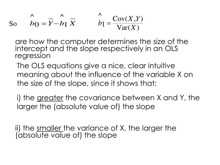
1. So are how the computer determines the size of the intercept and the slope respectively in an OLS regression The OLS equations give a nice, clear intuitive meaning about the influence of the variable X on the size of the slope, since it shows that: i) the greater the covariance between X and Y, the larger the (absolute value of) the slope ii) the smaller the variance of X, the larger the (absolute value of) the slope

2. It is equally important to be able to interpret the effect of an estimated regression coefficient Given OLS essentially passes a straight line through the data, then given Y = b0 + b1X So the OLS estimate of the slope will give an estimate of the unit change in the dependent variable y following a unit change in the level of the explanatory variable (so you need to be aware of the units of measurement of your variables in order to be able to interpret what the OLS coefficient is telling you)

3. PROPERTIES OF OLS Using the fact that for any individual observation, i, the ols residual is the difference between the actual and predicted value Sub. in So that Summing over all N observations in the data set and dividing by N 6

4. Since the sum of any series divided by the sample size gives the mean, can write and since So the mean value of the OLS residuals is zero (as any residual should be, since random and unpredictable by definition) 6

5. The 2nd useful property of OLS is that the mean of the OLS predicted values equals the mean of the actual values in the data (so OLS predicts average behaviour in the data set – another useful property)

6. Since the sum of any series divided by the sample size gives the mean, can write and since So the mean value of the OLS residuals is zero (as any residual should be, since random and unpredictable by definition) 6

7. Proof: summing Dividing by N We know from above that so

8. Story so far…… • Looked at idea behind OLS – fit a straight line thru the data that gives the “best fit” • Do this by choosing a value for the intercept and the slope of the straight line that will minimise the sum of squared residuals • OLS formula to do this given by

9. Things to do in Lecture 3 Useful algebra results underlying OLS Invent a summary measure of how well regression fits the data (R2) Look at contribution of individual variables in explaining outcomes, (Bias, Efficiency)

10. Useful Algebraic aspects of OLS and since So the mean value of the OLS residuals is zero (as any residual should be, since random and unpredictable by definition) 6

11. Proof: summing Dividing by N We know from above that so OLS predicts average behaviour

12. The 3rd useful result is that the covariance between the fitted values of Y and the residuals must be zero. 22

13. GOODNESS OF FIT Now we know how to summarise the relationships in the data using the OLS method, we next need a summary measure of “how well” the estimated OLS line fits the data Think of the dispersion of all possible y values (the variation in Y) being represented by a circle And similarly the dispersion in the range of x values Y X

14. The more the circles overlap the more the variation in the X data explains the variation in y Y Y X X Little overlap in values so X not explain much of variation in Y Large overlap in values so X variable explains much of variation in Y

15. To derive a statistical measure which does much the same thing remember that Using the rules on covariances (see problem set 0) we know that So the variation in the variable of interest, var(Y), is explained by either the variation in the variables included in the OLS model, or by variation in the residual 29

16. So we use the ratio As a measure of how well the model fits the data. (R2 is also known as the coefficient of determination) So R2 measures the % of variation in the dependent variable explained by the model. If the model explains all the variation in y then the ratio equals 1 So the closer the ratio is to one the better the fit.

17. It is more common however to use one further algebraic adjustment. Given (1) says that Can write this as The 1/n is common to both sides, so can cancel out and using the results that Then we have 29

18. The left side of the equation is the sum of the squared deviations of Y about its sample mean. This is called the Total Sum of Squares. The right hand side consists of the sum of squared deviations of the predictions around the sample mean (the Explained Sum of Squares) and the Residual Sum of Squares From this can have an alternative definition of the goodness of fit 29

19. Can see from above that it must hold that 0<= R2 <=1 when ESS = 0, then R2 = 0 (and model explains none of the variation in the dependent variable) when ESS = TSS, then R2 = 1 (and model explains all of the variation in the dependent variable) In general the R2 lies between these two extremes. You will find that for cross-section data (ie samples of individuals, firms etc) the R2 are typically in the region of 0.2 for time-series data (ie samples of aggregate (whole economy) data measured at different points in time) the R2 are typically in the region of 0.9

20. Why? Cross section data typically are bigger and have a lot more variation while time series data sets are smaller and have less variation in the dependent variable (easier to fit a straight line if data don’t vary much) While we would like the R2 to be as high as possible you can only compare R2 in models with the SAME dependent (Y) variable, so can’t say one model is a better fit than another if dependent variables are different

21. GOODNESS OF FIT So the R2 measures the proportion of variance in the dependent variable explained by the model Another useful interpretation of the R2 is that it equals the square of the correlation coefficient between the actual and predicted values of Y Proof: We know the formula for the correlation coefficient Sub. In for (actual value = predicted value plus residual ) 43

22. GOODNESS OF FIT Expand the covariance terms (since already proved And can always write any variance term as square root of the product 43

23. GOODNESS OF FIT Cancelling terms so Thus the correlation coefficient is the square root of R2. Eg R2 =0.25 implies correlation coefficient between Y variable & X variable (or between Y and predicted values ) = √0.25 = 0.5 43