Understanding Arrays and Structures: Abstract Data Types and Implementation

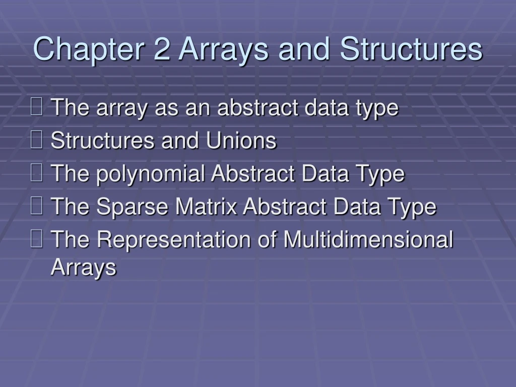
Chapter 2 Arrays and Structures • The array as an abstract data type • Structures and Unions • The polynomial Abstract Data Type • The Sparse Matrix Abstract Data Type • The Representation of Multidimensional Arrays

2.1 The array as an ADT (1/6) • Arrays • Array: a set of pairs, <index, value> • data structure • For each index, there is a value associated with that index. • representation (possible) • Implemented by using consecutive memory. • In mathematical terms, we call this a correspondence or a mapping.

2.1 The array as an ADT (2/6) • When considering an ADT we are more concerned with the operations that can be performed on an array. • Aside from creating a new array, most languages provide only two standard operations for arrays, one that retrieves a value, and a second that stores a value. • Structure 2.1 shows a definition of the array ADT • The advantage of this ADT definition is that it clearly points out the fact that the array is a more general structure than “a consecutive set of memory locations.”

2.1 The array as an ADT (3/6)

2.1 The array as an ADT (4/6) • Arrays in C • int list[5], *plist[5]; • list[5]: (five integers) list[0], list[1], list[2], list[3], list[4] • *plist[5]: (five pointers to integers) • plist[0], plist[1], plist[2], plist[3], plist[4] • implementation of 1-D arraylist[0] base address = list[1]  + sizeof(int)list[2]  + 2*sizeof(int)list[3]  + 3*sizeof(int)list[4]  + 4*sizeof(int)

2.1 The array as an ADT (5/6) • Arrays in C (cont’d) • Compare int *list1 and int list2[5] in C.Same: list1 and list2 are pointers.Difference: list2 reserves five locations. • Notations:list2 － a pointer to list2[0](list2 + i) － a pointer to list2[i] (&list2[i])*(list2 + i) － list2[i]

2.1 The array (6/6) • Example: 1-dimension array addressing • int one[] = {0, 1, 2, 3, 4}; • Goal: print out address and value • void print1(int *ptr, int rows){/* print out a one-dimensional array using a pointer */ int i; printf(“Address Contents\n”); for (i=0; i < rows; i++) printf(“%8u%5d\n”, ptr+i, *(ptr+i)); printf(“\n”);}

2.2 Structures and Unions (1/6) • 2.2.1 Structures (records) • Arrays are collections of data of the same type. In C there is an alternate way of grouping data that permit the data to vary in type. • This mechanism is called the struct, short for structure. • A structure is a collection of data items, where each item is identified as to its type and name.

2.2 Structures and Unions (2/6) • Create structure data type • We can create our own structure data types by using the typedef statement as below: • This says that human_being is the name of the type defined by the structure definition, and we may follow this definition with declarations of variables such as: • human_being person1, person2;

2.2 Structures and Unions (3/6) • We can also embed a structure within a structure. • A person born on February 11, 1994, would have have values for the datestruct set as

2.2 Structures and Unions (4/6) • 2.2.2 Unions • A union declaration is similar to a structure. • The fields of a union must share their memory space. • Only one field of the union is “active” at any given time • Example: Add fields for male and female. person1.sex_info.sex = male; person1.sex_info.u.beard = FALSE; and person2.sex_info.sex = female; person2.sex_info.u.children = 4;

2.2 Structures and Unions (5/6) • 2.2.3 Internal implementation of structures • The fields of a structure in memory will be stored in the same way using increasing address locations in the order specified in the structure definition. • Holes or padding may actually occur • Within a structure to permit two consecutive components to be properly aligned within memory • The size of an object of a struct or union type is the amount of storage necessary to represent the largest component, including any padding that may be required.

a b c 2.2 Structures and Unions (6/6) • 2.2.4 Self-Referential Structures • One or more of its components is a pointer to itself. • typedef struct list { char data; list *link; } • list item1, item2, item3;item1.data=‘a’;item2.data=‘b’;item3.data=‘c’;item1.link=item2.link=item3.link=NULL; Construct a list with three nodes item1.link=&item2; item2.link=&item3; malloc: obtain a node (memory) free: release memory

2.3 The polynomial ADT (1/10) • Ordered or Linear List Examples • ordered (linear) list: (item1, item2, item3, …, itemn) • (Sunday, Monday, Tuesday, Wednesday, Thursday, Friday, Saturday) • (Ace, 2, 3, 4, 5, 6, 7, 8, 9, 10, Jack, Queen, King) • (basement, lobby, mezzanine, first, second) • (1941, 1942, 1943, 1944, 1945) • (a1, a2, a3, …, an-1, an)

2.3 The polynomial ADT (2/10) • Operations on Ordered List • Finding the length, n , of the list. • Reading the items from left to right (or right to left). • Retrieving the i’th element. • Storing a new value into the i’th position. • Inserting a new element at the position i , causing elements numbered i, i+1, …, n to become numbered i+1, i+2, …, n+1 • Deleting the element at position i , causing elements numbered i+1, …, n to become numbered i, i+1, …, n-1 • Implementation • sequential mapping (1)~(4) • non-sequential mapping (5)~(6)

2.3 The polynomial ADT (3/10) • Polynomial examples: • Two example polynomials are: • A(x) = 3x20+2x5+4 and B(x) = x4+10x3+3x2+1 • Assume that we have two polynomials, A(x) = aixi and B(x) = bixiwhere x is the variable, aiis the coefficient, and i is the exponent,then: • A(x) + B(x) = (ai + bi)xi • A(x) · B(x) = (aixi · (bjxj)) • Similarly, we can define subtraction and division on polynomials, as well as many other operations.

2.3 The polynomial ADT (4/10) • An ADT definition of a polynomial

2.3 The polynomial ADT (5/10) • There are two ways to create the type polynomial in C • Representation I • define MAX_degree 101 /*MAX degree of polynomial+1*/typedef struct{ int degree; float coef [MAX_degree];}polynomial; drawback: the first representation may waste space.

2.3 (6/10) • Polynomial Addition • /* d =a + b, where a, b, and d are polynomials */d = Zero( )while (! IsZero(a) && ! IsZero(b)) do { switch COMPARE (Lead_Exp(a), Lead_Exp(b)) { case -1: d = Attach(d, Coef (b, Lead_Exp(b)), Lead_Exp(b)); b = Remove(b, Lead_Exp(b)); break; case 0: sum = Coef (a, Lead_Exp (a)) + Coef ( b, Lead_Exp(b)); if (sum) { Attach (d, sum, Lead_Exp(a)); } a = Remove(a , Lead_Exp(a)); b = Remove(b , Lead_Exp(b)); break; case 1: d = Attach(d, Coef (a, Lead_Exp(a)), Lead_Exp(a)); a = Remove(a, Lead_Exp(a)); } }insert any remaining terms of a or b into d *Program 2.4 :Initial version of padd function(p.62) advantage: easy implementation disadvantage: waste space when sparse

2.3 The polynomial ADT (7/10) • Representation II • MAX_TERMS 100 /*size of terms array*/typedef struct{ float coef; int expon;}polynomial;polynomial terms [MAX_TERMS];int avail = 0;

2.3 The polynomial ADT (8/10) • Use one global array to store all polynomials • Figure 2.2 shows how these polynomials are stored in the array terms. specification representation poly <start, finish> A <0,1> B <2,5> A(x) = 2x1000+1 B(x) = x4+10x3+3x2+1 storage requirements: start, finish, 2*(finish-start+1) non-sparse: twice as much as Representation I when all the items are nonzero

2.3 The polynomial ADT (9/10) • We would now like to write a C function that adds two polynomials, A and B, represented as above to obtain D = A + B. • To produce D(x),padd (Program 2.5) adds A(x) and B(x) term by term. Analysis: O(n+m) where n(m) is the number of nonzeros in A(B).

2.3 The polynomial ADT (10/10) Problem: Compaction is required when polynomials that are no longer needed. (data movement takes time.)

sparse matrix data structure? 2.4 The sparse matrix ADT (1/18) • 2.4.1 Introduction • In mathematics, a matrix contains m rows and n columns of elements, we write mn to designate a matrix with m rows and n columns. 5*3 6*6 15/15 8/36

2.4 The sparse matrix ADT (2/18) • The standard representation of a matrix is a two dimensional array defined as a[MAX_ROWS][MAX_COLS]. • We can locate quickly any element by writing a[i ][ j ] • Sparse matrix wastes space • We must consider alternate forms of representation. • Our representation of sparse matrices should store only nonzero elements. • Each element is characterized by<row, col, value>.

2.4 The sparse matrix ADT (3/18) • Structure 2.3 contains our specification of the matrix ADT. • A minimal set of operations includes matrix creation, addition, multiplication, and transpose.

2.4 The sparse matrix ADT (4/18) • We implement the Create operation as below:

2.4 The sparse matrix ADT (5/18) • Figure 2.4(a) shows how the sparse matrix of Figure 2.3(b) is represented in the array a. • Represented by a two-dimensional array. • Each element is characterized by <row, col, value>. # of rows (columns) # of nonzero terms transpose row, column in ascending order

2.4 The sparse matrix ADT (6/18) • 2.4.2 Transpose a Matrix • For each row i • take element <i, j, value> and store it in element <j, i, value> of the transpose. • difficulty: where to put <j, i, value>(0, 0, 15) ====> (0, 0, 15)(0, 3, 22) ====> (3, 0, 22)(0, 5, -15) ====> (5, 0, -15)(1, 1, 11) ====> (1, 1, 11)Move elements down very often. • For all elements in column j, place element <i, j, value> in element <j, i, value>

2.4 The sparse matrix ADT (7/18) • This algorithm is incorporated in transpose (Program 2.7). columns elements Scan the array “columns” times. The array has “elements” elements. ==> O(columns*elements)

2.4 The sparse matrix ADT (8/18) • Discussion: compared with 2-D array representation • O(columns*elements) vs. O(columns*rows) • elements --> columns * rows when non-sparse,O(columns2*rows) • Problem: Scan the array “columns” times. • In fact, we can transpose a matrix represented as a sequence of triples in O(columns + elements) time. • Solution: • First, determine the number of elements in each column of the original matrix. • Second, determine the starting positions of each row in the transpose matrix.

2.4 The sparse matrix ADT (9/18) • Compared with 2-D array representation: O(columns+elements)vs. O(columns*rows) elements --> columns * rows O(columns*rows) Cost:Additional row_terms and starting_pos arrays are required. Let the two arrays row_terms and starting_pos be shared. columns elements columns columns elements

2.4 The sparse matrix ADT (10/18) • After the execution of the third for loop, the values of row_terms and starting_pos are: [0] [1] [2] [3] [4] [5]row_terms = 21 2 2 0 1starting_pos = 1 3 4 6 8 8 transpose

2.4 The sparse matrix ADT (11/18) • 2.4.3 Matrix multiplication • Definition: • Given A and B where A is mn and B is np, the product matrix D has dimension mp. Its <i, j> element is • for 0  i < m and 0  j < p. • Example:

2.4 The sparse matrix ADT (12/18) • Sparse Matrix Multiplication • Definition: [D]m*p=[A]m*n* [B]n*p • Procedure: Fix a row of A and find all elements in column j of B for j=0, 1, …, p-1. • Alternative 1.Scan all of B to find all elements in j. • Alternative 2.Compute the transpose of B. (Put all column elements consecutively) • Once we have located the elements of row i of A and column j of B we just do a merge operation similar to that used in the polynomial addition of 2.2

2.4 The sparse matrix ADT (13/18) • General case: dij=ai0*b0j+ai1*b1j+…+ai(n-1)*b(n-1)j • Array A is grouped by i, and after transpose, array B is also grouped by j a Sa d Sd b Sb e Se c Sc f Sf g Sg The generation at most: entries ad, ae, af, ag, bd, be, bf, bg, cd, ce, cf, cg

The sparse matrix ADT (14/18) • An Example A = 1 0 2 BT = 3 -1 0 B = 3 0 2 -1 4 6 0 0 0 -1 0 0 2 0 5 0 0 5 a[0] 2 3 5 bt[0] 3 3 4 b[0] 3 3 4 [1] 00 1 bt[1] 00 3 b[1] 00 3 [2] 02 2 bt[2] 01 -1 b[2] 02 2 [3] 10 -1 bt[3] 20 2 b[3] 10 -1 [4] 1 1 4 bt[4] 2 2 5 b[4] 2 2 5 [5] 1 2 6 row col value row col value row col value

2.4 The sparse matrix ADT (15/18) • The programs 2.9 and 2.10 can obtain the product matrix D which multiplies matrices A and B. a × b

2.4 The sparse matrix ADT (16/18)

2.4 The sparse matrix ADT (17/18) • Analyzing the algorithm • cols_b * termsrow1 + totalb +cols_b * termsrow2 + totalb +… +cols_b * termsrowp + totalb= cols_b * (termsrow1 + termsrow2 + … + termsrowp)+rows_a * totalb= cols_b * totala + row_a * totalbO(cols_b * totala + rows_a * totalb)

2.4 The sparse matrix ADT (18/18) • Compared with matrix multiplication using array • for (i =0; i < rows_a; i++) for (j=0; j < cols_b; j++) { sum =0; for (k=0; k < cols_a; k++) sum += (a[i][k] *b[k][j]); d[i][j] =sum; } • O(rows_a * cols_a * cols_b) vs. O(cols_b * total_a + rows_a * total_b) • optimal case:total_a < rows_a * cols_a total_b < cols_a * cols_b • worse case:total_a --> rows_a * cols_a, or total_b --> cols_a * cols_b

2.5 Representation of multidimensional array (1/5) • The internal representation of multidimensional arrays requires more complex addressing formula. • If an array is declared a[upper0][upper1]…[uppern], then it is easy to see that the number of elements in the array is: • Where  is the product of the upperi’s. • Example: • If we declare a as a[10][10][10], then we require 10*10*10 = 1000 units of storage to hold the array.

2.5 Representation of multidimensional array (2/5) • Represent multidimensional arrays: row major order and column major order. • Row major order stores multidimensional arrays by rows. • A[upper0][upper1] as upper0 rows, row0, row1, …, rowupper0-1, each row containing upper1 elements.

2.5 Representation of multidimensional array (3/5) • Row major order: A[i][j] :  + i*upper1 + j • Column major order: A[i][j] :  + j*upper0 + i • col0 col1colu1-1 • row0 A[0][0] A[0][1] . . . A[0][u1-1] •  + u0+(u1-1)* u0 • row1 A[1][0] A[1][1] . . . A[1][u1-1] •  + u1 • . . . • rowu0-1 A[u0-1][0] A[u0-1][1] . . . A[u0-1][u1-1] • +(u0-1)*u1

2.5 Representation of multidimensional array (4/5) • To represent a three-dimensional array, A[upper0][upper1][upper2], we interpret the array as upper0 two-dimensional arrays of dimension upper1upper2. • To locate a[i][j][k], we first obtain  + i*upper1*upper2as the address of a[i][0][0] because there are i two dimensional arrays of size upper1*upper2 preceding this element. •  + i*upper1*upper2+j *upper2+k • as the address of a[i][j][k].

2.5 Representation of multidimensional array (5/5) • Generalizing on the preceding discussion, we can obtain the addressing formula for any element A[i0][i1]…[in-1] in an n-dimensional array declared as: A[upper0][upper1]…[uppern-1] • The address for A[i0][i1]…[in-1] is:

2.6 The String Abstract data type(1/19) 2.6.1 Introduction • The String: component elements are characters. • A string to have the form, S = s0, …, sn-1, where si are characters taken from the character set of the programming language. • If n = 0, then S is an empty or null string. • Operations in ADT 2.4, p. 81

2.6 The String Abstract data type(2/19) • ADT String:

2.6 The String Abstract data type(3/19) • In C, we represent strings as character arrays terminated with the null character \0. • Figure 2.8 shows how these strings would be represented internally in memory.

2.6 The String Abstract data type(4/19) • Now suppose we want to concatenate these strings together to produce the new string: • Two strings are joined together by strcat(s, t), which stores the result in s. Although s has increased in length by five, we have no additional space in s to store the extra five characters. Our compiler handled this problem inelegantly: it simply overwrote the memory to fit in the extra five characters. Since we declared t immediately after s, this meant that part of the word “house” disappeared.

Understanding Arrays and Structures: Abstract Data Types and Implementation