Download
1 / 64
650 likes | 876 Views
Informed Search. Uninformed searches easy but very inefficient in most cases of huge search tree Informed searches uses problem-specific information to reduce the search tree into a small one resolve time and memory complexities. Informed (Heuristic) Search. Best-first search

E N D
Informed Search • Uninformed searches • easy • but very inefficient in most cases of huge search tree • Informed searches • uses problem-specific information to reduce the search tree into a small one • resolve time and memory complexities
Informed (Heuristic) Search • Best-first search • It uses an evaluation function, f(n) • to determine the desirability of expanding nodes, making an order • The order of expanding nodes is essential • to the size of the search tree • less space, faster
Best-first search • Every node is then • attached with a value stating its goodness • The nodes in the queue are arranged • in the order that the best one is placed first • However this order doesn't guarantee • the node to expand is really the best • The node only appears to be best • because, in reality, the evaluation is not omniscient
Best-first search • The path cost g is one of the example • However, it doesn't direct the search toward the goal • Heuristic function h(n) is required • Estimate cost of the cheapest path • from node n to a goal state • Expand the node closest to the goal • = Expand the node with least cost • If n is a goal state, h(n) = 0
Greedy best-first search • Tries to expand the node • closest to the goal • because it’s likely to lead to a solution quickly • Just evaluates the node n by • heuristic function: f(n) = h(n) • E.g., SLD – Straight Line Distance • hSLD
Greedy best-first search • Goal is Bucharest • Initial state is Arad • hSLD cannot be computed from the problem itself • only obtainable from some amount of experience
Greedy best-first search • It is good ideally • but poor practically • since we cannot make sure a heuristic is good • Also, it just depends on estimates on future cost
Analysis of greedy search • Similar to depth-first search • not optimal • incomplete • suffers from the problem of repeated states • causing the solution never be found • The time and space complexities • depends on the quality of h
Properties of greedy best-first search • Complete? No – can get stuck in loops, e.g., Iasi Neamt Iasi Neamt • Time?O(bm), but a good heuristic can give dramatic improvement • Space?O(bm) -- keeps all nodes in memory • Optimal? No
A* search • The most well-known best-first search • evaluates nodes by combining • path cost g(n) and heuristic h(n) • f(n) = g(n) + h(n) • g(n) – cheapest known path • f(n) – cheapest estimated path • Minimizing the total path cost by • combining uniform-cost search • and greedy search
A* search • Uniform-cost search • optimal and complete • minimizes the cost of the path so far, g(n) • but can be very inefficient • greedy search + uniform-cost search • evaluation function is f(n) = g(n) + h(n) • [evaluated so far + estimated future] • f(n) = estimated cost of the cheapest solution through n
Analysis of A* search • A* search is • complete and optimal • time and space complexities are reasonable • But optimality can only be assured when • h(n) is admissible • h(n) never overestimates the cost to reach the goal • we can underestimate • hSLD, overestimate?
Optimality of A* A* has the following properties: The tree-search version of A* is optimal if h(n) is admissible, while the graph version is optimal if h(n) is consistent. * If h(n) is consistent then the values of f(n) along any path are nondecreasing.
Admissible heuristics • A heuristic h(n) is admissible if for every node n, • h(n) ≤ h*(n), where h*(n) is the true cost to reach the goal state from n. • An admissible heuristic never overestimates the cost to reach the goal, i.e., it is optimistic • Example: hSLD(n) (never overestimates the actual road distance) • Theorem: If h(n) is admissible, A* using TREE-SEARCH is optimal
Memory bounded search • Memory is another issue besides the time constraint • even more important than time • because a solution cannot be found if not enough memory is available • A solution can still be found • even though a long time is needed
Iterative deepening A* search • IDA* • = Iterative deepening (ID) + A* • As ID effectively reduces memory constraints • complete • and optimal • because it is indeed A* • IDA* uses f-cost(g+h) for cutoff • rather than depth • the cutoff value is the smallest f-cost of any node • that exceeded the cutoff value on the previous iteration
RBFS • Recursive best-first search • similar to depth-first search • which goes recursively in depth • except RBFS keeps track of f-value of the best alternative path available from any ancestor of the current node. • It remembers the best f-value • in the forgotten subtrees • if necessary, re-expand the nodes
RBFS • optimal • if h(n) is admissible • space complexity is: O(bd) • IDA* and RBFS suffer from • using too little memory • just keep track of f-cost and some information • Even if more memory were available, • IDA* and RBFS cannot make use of them
Simplified memory A* search • Weakness of IDA* and RBFS • only keeps a simple number: f-cost limit • This may be trapped by repeated states • IDA* is modified to SMA* • the current path is checked for repeated states • but unable to avoid repeated states generated by alternative paths • SMA* uses a history of nodes to avoid repeated states
Simplified memory A* search • SMA* has the following properties: • utilize whatever memory is made available to it • avoids repeated states as far as its memory allows, by deletion • complete if the available memory • is sufficient to store the shallowest solution path • optimal if enough memory • is available to store the shallowest optimal solution path
Simplified memory A* search • Otherwise, it returns the best solution that • can be reached with the available memory • When enough memory is available for the entire search tree • the search is optimally efficient • When SMA* has no memory left • it drops a node from the queue (tree) that is unpromising (seems to fail)
Simplified memory A* search • To avoid re-exploring, similar to RBFS, • it keeps information in the ancestor nodes • about quality of the best path in the forgotten subtree • If all other paths have been shown to be worse than the path it has forgotten Then it regenerates the forgotten subtree • SMA* can solve more difficult problems than A* (larger tree)
Simplified memory A* search • However, SMA* has to • repeatedly regenerate the same nodes for some problem • The problem becomes intractablefor SMA* • even though it would be tractable for A*, with unlimited memory • (it takes too long time!!!)
Heuristic functions • For the problem of 8-puzzle • two heuristic functions can be applied • to cut down the search tree • h1 = the number of misplaced tiles • h1 is admissible because it never overestimates • at least h1 steps to reach the goal.
Heuristic functions • h2= the sum of distances of the tiles from their goal positions • This distance is called city block distance or Manhattan distance • as it counts horizontally and vertically • h2 is also admissible, in the example: • h2 = 3 + 1 + 2 + 2 + 2 + 3 + 3 + 2 = 18 • True cost = 26
The effect of heuristic accuracy on performance • effective branching factorb* • can represent the quality of a heuristic • IF N= the total number of nodes expanded by A* and the solution depth is d, THEN b* is the branching factor of the uniform tree • N = 1 + b* + (b*)2 + …. + (b*)d • N is small if b* tends to 1
The effect of heuristic accuracy on performance • h2dominatesh1 if for any node, h2(n) ≥ h1(n) • Conclusion: • always better to use a heuristic function with higher values, as long as it does not overestimate
Inventing admissible heuristic functions • relaxed problem • A problem with less restriction on the operators • It is often the case that • the cost of an exact solution to a relaxed problem • is a good heuristic for the original problem
Inventing admissible heuristic functions • Original problem: • A tile can move from square A to square B • if A is horizontally or vertically adjacent to B and B is blank • Relaxed problem: • A tile can move from square A to square B • if A is horizontally or vertically adjacent to B • A tile can move from square A to square B • if B is blank • A tile can move from square A to square B
Inventing admissible heuristic functions • If one doesn't know the “clearly best” heuristic • among the h1, …, hm heuristics • then set h(n) = max(h1(n), …, hm(n)) • i.e., let the computer run it • Determine at run time
Generating admissible heuristic from subproblem • Admissible heuristic • can also be derived from the solution cost of a subproblem of a given problem • getting only 4 tiles into their positions • cost of the optimal solution of this subproblem • used as a lower bound
Local search algorithms • So far, we are finding solution paths by searching (Initial state goal state) • In many problems, however, • the path to goal is irrelevant to solution • e.g., 8-queens problem • solution • the final configuration • not the order they are added or modified • Hence we can consider other kinds of method • Local search
Local search • Just operate on a single current state • rather than multiple paths • Generally move only to • neighbors of that state • The paths followed by the search • are not retained • hence the method is not systematic
Local search • Two advantages : 1. uses little memory – a constant amount • for current state and some information 2. can find reasonable solutions • in large or infinite (continuous) state spaces • where systematic algorithms are unsuitable • Also suitable for • optimization problems in which the aim is to find the best state according to an objective function
Local search • State space landscape has two axis • location (defined by states) • elevation (defined by objective function or by the value of heuristic cost function)
Local search • If elevation corresponds to cost then, the aim is to find lowest valley( global minimum). • If elevation corresponds to an objective function, then the aim is to find highest peak( global maximum).
Local search • A complete local search algorithm • always finds a goal if one exists • An optimal algorithm • always finds a global maximum/minimum
Hill-climbing search(greedy local search) • simply a loop • It continually moves in the direction of increasing value • i.e., uphill • No search tree is maintained • The node need only record • the state • its evaluation (value, real number)
Hill-climbing search • Evaluation function calculates • the cost • a quantity instead of a quality • When there is more than one best successor to choose from • the algorithm can select among them at random
Drawbacks of Hill-climbing search Hill-climbing is also called • greedy local search • grabs a good neighbor state • without thinking about where to go next. *** Hill-climbing often gets stuck for the following reasons:- • Local maxima: • The peaks lower than the highest peak in the state space • The algorithm stops even though the solution is far from satisfactory
Drawbacks of Hill-climbing search • Ridges • The grid of states is overlapped on a ridge rising from left to right • Unless there happen to be operators • moving directly along the top of the ridge • the search may oscillate from side to side, making little progress
Drawbacks of Hill-climbing search • Plateaux • an area of the state space landscape • where the evaluation function is flat • shoulder • impossible to make progress • Hill-climbing might be unable to • find its way off the plateau