Download
1 / 26
270 likes | 654 Views
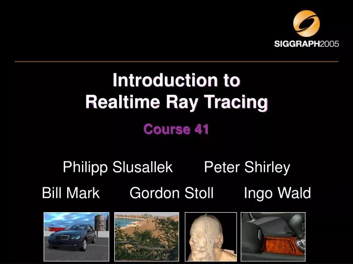
Introduction to Realtime Ray Tracing Course 41. Philipp Slusallek Peter Shirley Bill Mark Gordon Stoll Ingo Wald. Ray Tracing. Highly Realistic Images Ray tracing enables correct simulation of light transport. Internet Ray Tracing Competition, June 2002.

E N D
Introduction to Realtime Ray TracingCourse 41 Philipp Slusallek Peter Shirley Bill Mark Gordon Stoll Ingo Wald
Ray Tracing • Highly Realistic Images • Ray tracing enables correct simulation of light transport Internet Ray Tracing Competition, June 2002
Ray Tracing of Surfaces • Assumption: empty space totally transparent • Surfaces • 3D geometry models of objects • Optical surface characteristics (Appearance) • Absorption, reflection, transparency, color, … • Illumination • Position, characteristics of light emitters
Fundamental Steps • Generation of primary rays • Rays from viewpoint into 3D scene • Ray tracing & traversal • First intersection with scene geometry • Shading • Light (radiance) send along primary ray • Compute incoming illumination with recursive rays
Ray Generation • Pinhole camera • o: Origin (point of view) • f: Vector to center of view, focal length • x, y: Span the viewing window • xres, yres: Image resolution x y d f u o
Ray Generation • Pinhole camera for (x= 0; x < xres; x++) for (y= 0; y < yres; y++) { d= f + 2(x/xres - 0.5)x + 2(y/yres - 0.5)y; d= d/|d|; // Normalize col= trace(o, d); write_pixel(x,y,col); } x y d f u o
Ray and Object Representations • Ray in space: r(t)=o+t d • o=(ox, oy, oz), d=(dx, dy, dz) • Scene geometry • Plane: (p-a)·n=0 • Implicit definition (n : surface normal, a : point one surface ) • Sphere: (p-c)·(p-c)-r2=0 • c : sphere center, r : sphere radius • Triangles: Plane plus 2D coordinates
R o d Intersection Ray -Sphere • Sphere • Given a sphere at the origin (x2 + y2 + z2 - 1= 0) • Substituting the ray into the equation gives t2(dx2 + dy2 + dz2) + 2t (dxox + dyoy + dzoz) + (ox2 + oy2 + oz2) –1 = 0 • Alternative: Geometric construction • Ray and center span a plane • Simple 2D construction
Intersection Ray - Plane • Plane • Plane Equation: p·n - D = 0, |n| = 1 • Implicit representation (Hesse form) • Normal vector: n • Normal distance from (0, 0, 0): D • Substitute o + td for p • (o + td)·n – D = 0 • Solving for t gives d o d·n n o·n D p
C 1 P 3 0 B A Intersection Ray - Triangle • Barycentric coordinates • Non-degenerate triangle ABCP= 1A + 2B + 3C • 1 + 2 + 3 = 1 • 3 = (APB) / (ACB) etc • Relative area • Hit iff all i greater or equal than zero
n Intersection Ray - Triangle • Compute intersection with triangle plane • Given the 3D intersection point • Project point into xy, xz, yz coordinate plane • Use coordinate plane that is most aligned • Coordinate plane and 2D vertices can be pre-computed • Perform barycentric test
Ray Tracing Acceleration • Intersect ray with all objects • Way too expensive • Faster intersection algorithms • Little effect • Less intersection computations • Space partitioning (often hierarchical) • Grid, octree, BSP or kd-tree, bounding volume hierarchy (BVH) • 5D partitioning (space and direction)
Grid • Building a grid structure • Start with bounding box • Resolution: often ~ 3n • Overlap or intersection test • Traversal • 3D-DDA • Stop if intersection found in current voxel
Grid: Issues • Grid traversal • Requires enumeration of voxel along ray 3D-DDA • Simple and hardware-friendly • Grid resolution • Strongly scene dependent • Cannot adapt to local density of objects • Problem: „Teapot in a stadium“ • Possible solution: hierarchical grids
Grid: Issues • Objects in multiple voxels • Store only references • Use mailboxing to avoid multiple intersection computations • Store (ray, object)-tuple in small cache (e.g. with hashing) • Do not intersect if found in cache • Original mailbox uses ray-id stored with each triangle • Simple, but likely to destroy CPU caches
History of Intersection Algorithms • Ray-geometry intersection algorithms • Polygons: [Appel ’68] • Quadrics, CSG: [Goldstein & Nagel ’71] • Recursive Ray Tracing: [Whitted ’79] • Tori: [Roth ’82] • Bicubic patches: [Whitted ’80, Kajiya ’82, Benthin ’04] • Algebraic surfaces: [Hanrahan ’82] • Swept surfaces: [Kajiya ’83, van Wijk ’84] • Fractals: [Kajiya ’83] • Deformations: [Barr ’86] • NURBS: [Stürzlinger ’98] • Subdivision surfaces: [Kobbelt et al ’98, Benthin ‘04] • Points [Schaufler et al.’00, Wald ’05]
Hierarchical Grids • Simple building algorithm • Recursively create grids in high-density voxels • Problem: What is the right resolution for each level? • Advanced algorithm • Separate grids for object clusters • Problem: What are good clusters?
Octree • Hierarchical space partitioning • Adaptively subdivide voxels into 8 equal sub-voxels recursively • Result in subdivision • Problems • Rather complex traversal algorithms • Slow to refine complexregions
Bounding Volumes • Idea • Only compute intersection if ray hits BV • Possible bounding volumes • Sphere • Axis-aligned box • Non-axis-aligned box • Slabs
Bounding Volume Hierarchies • Idea: • Apply recursively • Advantages: • Very good adaptivity • Efficient traversal O(log N) • Problems • How to arrange BVs?
BSP- and Kd-Trees • Recursive space partitioning with half-spaces • Binary Space Partition (BSP): • Splitting with half-spaces in arbitrary position • Kd-Tree • Splitting with axis-aligned half-spaces 1.1.2 1.1.2.1 1 1.2 1.1 1.1.1 1.1.1.1
Ray Differentials [Homan Igehy, Siggraph99] • Path Differentials [Frank Suykens, EGRW’01]
Siggraph 2005:More Realtime Ray Tracing • Introduction to Realtime Ray Tracing • Full day course: Wednesday, Petree Hall D • Booth 1155: Mercury Computer Systems • Realtime ray tracing product on PC clusters • Realtime ray tracing on the Cell Processor • Realtime previewing in Cinema-4D • Booth 1511: SGI • Ray tracing massive model : Boeing 777