Download

1 / 45
450 likes | 580 Views
Motion Planning. By Gene Peterson. CS 6160, Spring 2010. 5/4/2010. What is Motion Planning?. Given a set of obstacles, a start position, and a destination position, find a path from start to destination that doesn’t go through any obstacles This project seeks shortest path

E N D
Motion Planning By Gene Peterson CS 6160, Spring 2010 5/4/2010
What is Motion Planning? • Given a set of obstacles, a start position, and a destination position, find a path from start to destination that doesn’t go through any obstacles • This project seeks shortest path • Many variations on the basic problem
Program • Two parts: Course builder and simulator • Course Builder: made in C# using XNA and Windows forms • User-friendly interface • Simulator: approximately 2000 lines of code • OpenGL rendering
Potential Project Goals • Point object path finding • Polygonal object finding • Robot rotation • Real-time calculation • Non-convex obstacles • Moving obstacles • Curves • No global vision • 3D problem • Path weighting • Group travel
Procedure • Define input: obstacles, “robot”, starting position, and destination • Create a visibility graph • Find the shortest path from start to destination in the graph
Required Geometry • Point • Vector • Line • Line Segment • Ray • Poly Line • Polygon
Defining a Polygon • Ordered set vertices • Edges implicitly defined by adjacency in the vertex list • May be clockwise or counter-clockwise wound
Open or Closed Polygons? Open Closed Does it matter?
Open vs Closed Polygon No Intersection Intersection
Open vs Closed Polygons • Cannot achieve shortest possible path with closed polygons • Always can get slightly closer • Open polygons cannot get any closer to the polygon without penetrating it
Course Builder • Create 2D polygons and lay them out as a course • Saved to file, loaded by simulator
Convex Hull Algorithm #1 • Trivial O(n^3) algorithm • Every pair of vertices is checked to see if it can be an edge of the convex set
Convex Hull Algorithm #2 • Gift wrapping technique • O(n*h) • n: # of vertices • h: # of vertices in the convex hull
Convex Hull Algorithm #3 • Graham-Schmidt algorithm • O(n log n) • n: # of vertices • Sorts the points • Didn’t attempt algorithm #4: mix of gift wrapping with Graham-Schmidt
Polygonal Robot • Instead of a point robot, use a polygon • By calculating the Configuration Space of the polygonal robot, the robot can be represented by a point • C-Space is the areas that the point robot cannot move
Configuration Space • Calculate C-Space version of each obstacle using Minkowski sum of the polygon and the robot
Minkowski Sum Algorithm #1 • Trivial algorithm - O(n^3) • For each vertex a in polygon A For each vertex b in polygon B Add point (a+b) to P • Minkowski sum is the convex hull of points P
Minkowski Sum Algorithm #2 • Sweep method – O(n + m) • n: # of vertices in polygon A • m: # of vertices in polygon B • Sorts the points in each polygon in counter-clockwise order • Next point is the point with smallest angle
Visibility Graph • Graph vertices represent vertices of the C-Space obstacles and the start and destination points • Edges represent possible paths • If a line segment from any vertex in the graph to any other vertex in the graph doesn’t penetrate an obstacle, there’s an edge between those two vertices • Edge weights represent distance between points • Shortest path in the graph is shortest path through the obstacles
Visibility Graph Algorithm #1 • O(n^3) • Create every possible line segment from pairs of vertices in the graph • Any line segment that doesn’t penetrate an obstacle gets added as an edge in the graph
Visibility Graph Algorithm #2 • O(n^2 log n) • Sweep algorithm • Uses the fact that some edges will obscure other edges from being visible • Requires a line segment search tree data structure
Ray-Line Segment AVG Tree • Balanced binary search tree • Given a ray, find the line segment in the tree that it will intersect first
Shortest Path • Now that we have an obstacle course and a visibility graph for it, we can calculate the shortest path using graph algorithms
Dijkstra’s Algorithm • Breadth first search with weights • Only non-negative edges • Requires priority queue
Path Finding in Video Games • Generally discretised (grid based) • 2D path finding useful in many 3D games • Speed important (1/60th of a second/frame) • Accuracy less important • Much of the environment is static • Precomputation often available
Precomputation • Precalculate visibility graph of C-Space obstacles only (don’t include any start or end point) • To create the full visibility graph, insert start and destination points (calculating visibility for each polygon vertex for them) • Use a copy of precalculated visibility graph so it can be reused • Needs to be recomputed as often as the environment changes
Statistics • TO FILL IN WHEN I HAVE THE FINAL STATISTICS AVAILABLE
More Speed? • Multi-threading • CUDA • Performance optimizations (length squared, etc) • Minimizing geometry where possible • Sacrifice accuracy • Amortize path finding cost over time
Robot Rotation • Unlike translation, rotating the robot changes the C-Space • Even if rotation angles are discretized, greatly enlarges the graph size, and thus the computation time • Gave up on this problem to pursue other aspects of motion planning
Goals Revisited • Point object path finding • Polygonal object finding • Robot rotation • Real-time calculation • Non-convex obstacles • Moving obstacles • Curves • No global vision • 3D problem • Path weighting • Group travel Too computationally expensive for real-time Not as useful in video games, slow Didn’t get to it Beyond the scope of this project AI Problem AI Problem
Further Exploration • Rotation • Better precomputation • Non-convex performance • Sacrificing accuracy for performance • Regional partitioning
Implicit Line Equation from 2 Points • Given two points on the line, calculate a, b, c Pick any a and b that make this true Use any point (x,y) on the line * Any multiple k ≠ 0 applied to (a, b, c) will result in the same line
Half Space (2D) • Input: Line and a Point • Output: Real (+,-,0) • Geometric Interpretation: 0 means the point is on the line + means on one side of the line - means on the other side • Plug point into implicit line equation • Result is the half space that contains the point (+,-,0)
Line-Line Intersection (2D) • Line 0: • Line 1: • Solve for (x,y): two equations, two unknowns • Three cases:- No intersection (parallel lines)- Always intersect (same line)- One intersection
Line-Line Intersection (2D) cont. • No intersection (parallel lines) • Always intersect (same line) • Otherwise, solve for (x,y) • Constant time Slope of the two lines are equal: But not the same line: For k ≠ 0:
Line Segment-Line Segment Intersection • Find intersection point using line-line intersection (if it exists, if it doesn’t the line segments don’t intersect) • Create a ray for each line segment • Ray ranges from 0 to 1 along the line segment • Calculate t of the intersection point for each line segment • If both t’s are in [0,1], line segments intersect
Point-Line Intersection • Calculate the halfspace the point lies in • If halfspace equals 0, point is on the line • Floating point error may play into this • Use an epsilon, point is near close enough to being on the line
Point-Polygon Intersection • Calculate the half space the point lies in for each edge of the polygon • If the polygon is clockwise wound, the point must always be in - half space • If the polygon is counter-clockwise wound, the point must always be in + half space • O(# of vertices in the polygon)
Clockwise Winding Counter-Clockwise Winding + - - + - - + + - + + - + - + -
Polygon-Polygon Intersection • Possibly intersecting or fully contained • Check each line segment in polygon A for intersection with each line segment in polygon B • Check for containment: pick a point from A and see if it’s in B (and do same check to see if B is in A)