Download

1 / 33
330 likes | 364 Views
Learn about spline interpolation techniques including linear, quadratic, and cubic splines. Explore the derivation process and implementation in MATLAB with examples. Understand the conditions and equations for fitting splines to data points.

E N D
Chapter 15 Curve Fitting : Splines Gab Byung Chae
Notation used to derive splines n-1 intervals in n data points
Splines in 1st, 2nd, 3rd order • Linear spline • Quadratic spline • Cubic spline
15.2 Linear Splines linear splines passing thru Example : (3,2.5),(4.5,1),(7,2.5),(9,.5) -> (5,?)
15.3 Quadratic Splines • The objective in quadratic splines is to derive a second-order polynomial for each interval between data points • The polynomial : si(x) =ai + bi(x-xi)+ ci(x-xi)2 For n data points, there are n-1 intervals and, consequently, 3(n-1) unknown constants to evaluate. 3(n-1) equations or conditions are required to evaluate the unknowns.
Let for all i=1,,..,n-1 1. Continuity condition : the function must pass through all the points. --- (15.6) for all i=1,,..,n-1 : (n-1) equations 2. The function values of adjacent polynomials must be equal at the knots. --- (15.8) for all i=1,,..,n-1 : (n-1) equations
Let for all i=1,,..,n-1 3. The first derivatives at the interior nodes must be equal. (n-2) eq.s --- (15.9) 4. Assume that the second derivative is zero at the first point. 1 equation Example : (3,2.5),(4.5,1),(7,2.5),(9,.5) -> (5,?)
Example 15.2 • Problem] Fit quadratic splines to the data in Table 15.1. Use the results to estimate the value at x=5.
Solution] Equation (15.8) is written for i=1 through 3 (with c1=0) to give f1+ b1h1 = f2 f2+ b2h2 + c2h22 = f3 f3+ b3h3 + c3h32 = f4 Equation (15.9) creates 2 conditions with c1=0 : b1 = b2 b2+ 2c2h2 = b3
f1 = 2.5 h1 = 4.5-3.0 = 1.5 • f2 = 1.0 h2 = 7.0-4.5 = 2.5 • f3 = 2.5 h3 = 9.0-7.0 = 2.0 • f4 = 0.5 2.5 + 1.5 b1 = 1.0 1.0 + 2.5 b2 + 6.25 c2 = 2.5 2.5 + 2.0 b3 + 4c3 = 0.5 b1 - b2 = 0 b2 - b3 + 5c2= 0
b1 = -1 b2 = -1 c2 = 0.64 b3= 2.2 c3 = -1.6 s1(x) = 2.5 –(x-3) s2(x) = 1.0 –(x-4.5)+0.64(x-4.5)2 s3(x) = 2.5 + 2.2(x-7.0)-1.6(5-7.0)2 x=5 이므로 s2(5) = 1.0 –(5-4.5)+0.64(5-4.5)2 =0.66
15.4 Cubic Splines a. (n-1) eq.s b. (n-1) eq.s c. (n-2) eq.s d. (n-2) eq.s e. 2 eq.s
Example 15.3 Fit cubic splines to the data . Utilize the results to estimate the value at x =5
Solution : employ Eq.(15.27) • f1 = 2.5 h1 = 4.5-3.0 = 1.5 • f2 = 1.0 h2 = 7.0-4.5 = 2.5 • f3 = 2.5 h3 = 9.0-7.0 = 2.0 • f4 = 0.5
So we have • Using MATLAB the results are • c1 = 0 c2 = 0.839543726 • c3 = -0.766539924 c4 = 0
Using Eq. (15.21) and (15.18), • b1 = -1.419771863 d1 = 0.186565272 • b2 = -0.160456274 d2 = -0.214144487 • b3 = 0.022053232 d3 = 0.127756654
15.4.2 End Conditions • Clamped End Condition : Specifying the first derivatives at the first and last nodes. • Not-a-Knot End Condition : Force continuity of the third derivative at the second and the next-to-last knots. – same cubic functions will apply to each of the first and last two adjacent segments,
15.5 Piecewise interpolation in Matlab 15.5.1 MATLAB function : spline • Syntax : yy = spline(x, y, xx)
Example 15.4 Splines in MATLAB • Use MATLAB to fit 9 equally spaced data points sampled from this function in the interval [-1, 1]. • a) a not-a-knot spline b) a clamped spline with end slopes of f1’=1 and f’n-1 = -4
Solution : a) >> x = linspace(-1,1,9); >> y = 1./(1+25*x.^2); >> xx = linspace(-1,1); >> yy = spline(x,y,xx); >> yr = 1./(1+25*xx.^2); >> plot(x,y,’o’,xx,yy,xx,yr,’—’)
b) >> yc =[1 y -4]; >> yyc =spline(x,yx,xx); >> plot(x,y,’o’,xx,yyc,xx,yr,’—’)
15.5.2 MATLAB function : interp1 • Implement a number of different types of piecewise one-dimensional interpolation. • Syntax : yi = interp1(x,y,xi, ‘method’) yi = a vector containing the results of the interpolation as evaluated at the points in the vector xi , and ‘method’ = the desired method.
method • Nearest – nearest neighbor interpolation. • Linear – linear interpolation • Spline – piecewise cubic spline interpolation(identical to the spline function) • pchip and cubic – piecewise cubic Hermite interpolation. • The default is linear.
MATLAB’s methods >> yy=spline(x,y,xx); cubic spilne >> yy=interp1(x,y,xx): (piecewise) linear spline >> yy=interp1(x,y,xx,’spline’): cubic spline >> yy=interp1(x,y,xx,’nearest’) : nearest neighbormethod >> yy=interp1(x,y,xx,’pchip’): piecewise cubic Hermite interpolation >> zz=interp2(x,y,z,xx,yy): 2 dimensional interpolation
Example 15.5 Trade-offs Using interpl • Linear, nearest, cubic spline, piecewise cubic Hermite interpolation
>> t = [ 0 20 40 56 68 80 84 96 104 110]; >> v = [0 20 20 38 80 80 100 100 125 125]; >> tt = linspace(0,110); >> vl=interp1(t,v,tt); %(piecewise) linear spline >> plot(t,v,’o’,tt,vl) >> vn=interp1(t,v,tt,’nearest’); % nearest >> plot(t,v,’o’,tt,vn) >> vs=interp1(t,v,tt,’spline’); % cubic spline >> plot(t,v,’o’,tt,vs) >> vh=interp1(t,v,tt,’pchip’); % piecewise cubic Hermite interpolation >> plot(t,v,’o’,tt,vh)