Download
1 / 15
170 likes | 342 Views
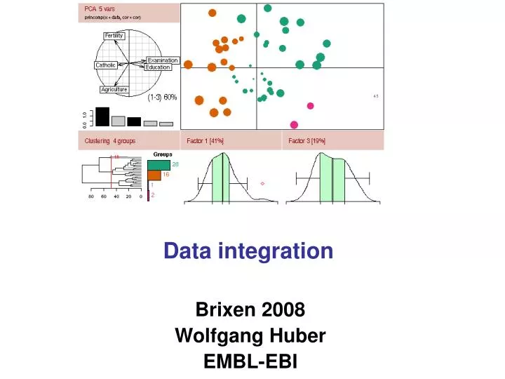
Data integration. Brixen 2008 Wolfgang Huber EMBL-EBI. Overview. Along genomic coordinates By gene (by pairs of genes) (by sets of genes) Here, "gene" is used in loose sense, to be defined as appropriate for the application; the concept encompasses: Loci on the DNA

E N D
Data integration Brixen 2008 Wolfgang Huber EMBL-EBI
Overview • Along genomic coordinates • By gene • (by pairs of genes) • (by sets of genes) • Here, "gene" is used in loose sense, to be defined as appropriate for the application; the concept encompasses: • Loci on the DNA • Transcripts (RNA molecules) • Proteins
Integration of data along genomic coordinates • An example: • We measured the frequency of recombination events (cross-overs, gene conversions not associated with crossover) throughout the genome of S cerevisiae. • Is this pattern ('hotspots') associated with: • GC content • promoters • across- or within species conservation CO NCO
Testing for association • You can consider the different sets of features along the genome as continuous-valued, or binary, "time" series • X1(t), ..., Xn(t) • Consider, e.g., the case where Xi(t) and Xj(t) are {0,1} indicators.A simple (but as we will see, inadequate) approach would be to compute an overlap statistic such as • or • and estimate its null distribution through random permutation in t.
Testing for association • Alternatively, one could also compute, for each feature in series i, the distance to the closest feature in j, and then take a summary of the distribution of that statistic (e.g. median).
"Boring" association of features in inhomogenous time series nearest neighbour distance: uniform genome genome with blocks
## Flawed testing for association along the genome • library("geneplotter") • library("RColorBrewer") • n = 10000 • oneplot = function(weights, s=200) { • e1 = sample(n, s, prob=weights) • e2 = sample(n, s, prob=weights) • d = matchpt(e1, e2)$distance • plot(x=e1, y=rep(1, length(e1)), type="p", pch=16, col= "#A6CEE3", ylim=c(-0.1, 1.1), xlab="", ylab="") • points(x=e2, y=rep(0.9, length(e2)), pch=16, col= "#B2DF8A") • lines(weights/sum(weights)*0.3, col="grey") • return(d) • } • w1 = rep(1, n) • w2 = rep(rep(c(0, 1), each=n/8), 4) • par(mfrow=c(3,1)) • dists = list( • w1=oneplot(w1), • w2=oneplot(w2)) • multidensity(dists, xlab="Distances", xlim=c(0, 120)) • legend("topright", names(dists), lwd=2, lty=1, col=brewer.pal(9, "Set1"))
Testing for association • "Everything is correlated with GC-content"; Etc. • Hence everything is correlated with everything else. That is not very interesting. • Are two sets of genomic features correlated more than expected? • To be interesting, this "expectation" is not just uniform random distribution along the genome, but includes some "background model". When setting up such a test, we need to define what an interesting background model (null hypothesis) is, then set up an appropriate randomization scheme to try to reject it. • For example, we could say that we know that there are long range structures in the genome, in which we are not interested, and we want to test whether two features that we mapped at fine scale show local correlation above the coarse-scale correlation.
Data integration via "genes" • A common and intuitive method for data integration is to compare the data from different experiments (assays) by mapping them all to the same set of genes. • This sounds easier than it is: different assays investigate different aspects of a gene • transcript(s) level • protein product(s) level, localization, structure, ... • chromatin state • promoter • UTRs • antisense transcript • and our understanding of how these aspects are organised together in a gene may be subtle, controversial, and changeable over time.
Data integration via "genes" • The reagents and target molecule identifiers used in different experiments may be different: • RefSeq ID • Entrez ID • Ensembl Gene ID • Ensembl Transcript ID • Uniprot ID • Gene coordinate on the chrosome • Microarray probe sequence • siRNA sequence • Peptide sequence identified in MS • Short Read Sequence • Bioconductor offers tools to map these to each other (annotation packages; biomaRt; Biostrings).
Data integration via "genes" • Bioconductor offers tools to map these to each other, so • others can reproduce your mapping • you can redo the mapping as the biological databases get updated • you can try out different ways to do the mapping and see how they affect the subsequent data analysis • Think about this early: • - keep the primary reagent identifiers around • - use versioning (annotation packages!) • - make the mapping process part of your reproducible, documented, automated workflow
Acknowledgement • Robert Gentleman • Richard Bourgon • Jörn Tödling • Greg Pau
Report Generation hwriter package
References • Visualizing Genomic Data, R. Gentleman, F. Hahne, W. Huber (2006), Bioconductor Project Working Papers, Paper 10 • Choosing Color Palettes for Statistical Graphics, A. Zeileis, K. Hornik (2006), Department of Statistics and Mathematics, Wirtschaftsuniversität Wien, Research Report Series, Report 41