Online Application Demos

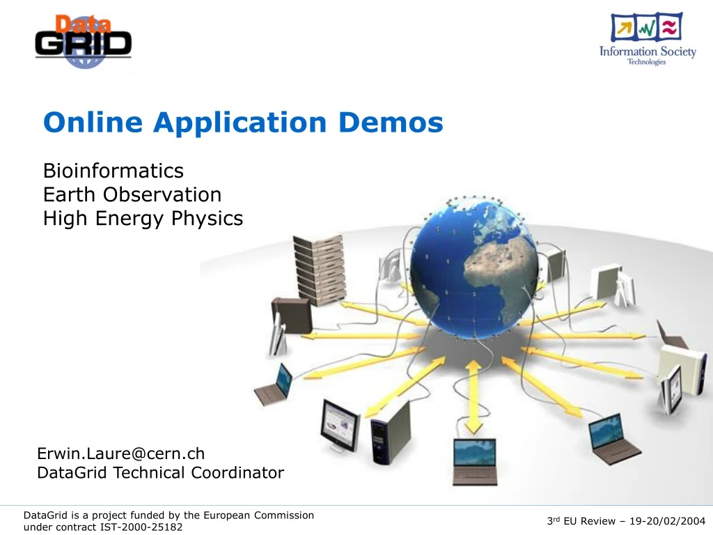
1. Online Application Demos BioinformaticsEarth ObservationHigh Energy Physics Erwin.Laure@cern.ch DataGrid Technical Coordinator

2. 4 Application Demos Monte-Carlo simulation for medical applications Metadata usage in ozone profile validation

3. Node A Node B Advanced Scheduling in HEP Applications: CMS demonstrating DAGMan scheduling Node D Node C Node E HEP production usage of Grid platforms: the ALICE project

4. Grid infrastructures used EDG application testbed INFN testbed LCG-2 infrastructure

5. Parallelization of Monte Carlo simulations GATE for medical applications The scenario of a typical radiotherapy treatment WP10 Lydia Maigne, Yannick Legré maigne@clermont.in2p3.fr legre@clermont.in2p3.fr

6. Radiotherapy is widely used to treat cancer 1°) Obtain scanner slices images 2°) Treatment planning 3°) Radiotherapy treatment The head is imaged using a MRI and/or CT scanner Calculation of deposit dose on the tumor (~1mn): A treatment plan is developed using the images Irradiation of the brain tumor with a linear accelerator

7. Ocular brachytherapy treatment PET camera Radiotherapy Better treatment requires better planning • Today: analytic calculation to compute dosedistributions in the tumor • For new Intensity Modulated Radiotherapy treatments, analytic calculations off by 10 to 20% near heterogeneities • Alternative: Monte Carlo (MC) simulations in medical applications • The GRID impact: reduce MC computing time to a few minutes WP10 Demo:gridification of GATE MC simulation platform on the DataGrid testbed

8. Computation of a radiotherapy treatment on the Datagrid: Let’s go….

9. Storage Element Storage Element Storage Element Storage Element Computing Element Computing Element Computing Element Computing Element GATE applications on the DataGrid Gabriel Montpied hospital, Clermont-Ferrand GATE Registration of the medical image on SE Copy of the medical image from SE to CE Submission on sites of the DataGrid Retrieving of root outputs on the UI Replication of the medical image on SEs Registration of lfns in the database CCIN2P3 GATE RAL Scanner slices: DICOM format GATE User interface NIKHEF Concatenation Anonymisation Database GATE Image: text file MARSEILLE Binary file: Image.raw Size: 19M

10. 1°) Obtain the medical images of the tumor: • 38 scanner slices of the brain of a patient are obtained Scanner slices: DICOM format • Format of the slices: • 512 X 512 X 1 pixels • Size of a voxel in the image: • 0,625 X 0,625 X 1,25 mm

11. 2°) Concatenate these slices in order to obtain a 3D matrix:Pixies software Scanner slices: DICOM format Concatenation

12. 3°) Transform the DICOM format of the image into an Interfile formatPixies software Binary image of the scanner slices Scanner slices: DICOM format Concatenation Size of the matrix Anonymisation Size of the pixels Image: text file Number of slices Binary file: Image.raw Size 19M

13. Storage Element Storage Element Storage Element Storage Element Computing Element Computing Element Computing Element Computing Element 4°) Register and replicate the binary image on SEs: Replicate lfns on the other SEs Copy image.raw on a SE CCIN2P3 Scanner slices: DICOM format RAL User interface Concatenation NIKHEF Anonymisation Image: text file MARSEILLE Binary file: Image.raw Size 19M Visualization

14. Storage Element Storage Element Storage Element Storage Element Computing Element Computing Element Computing Element Computing Element 5°) Register the lfn of an image: • WP2 spitfire or local database CCIN2P3 Query a lfn to the database Register lfn in the database Scanner slices: DICOM format RAL User interface Concatenation NIKHEF Anonymisation Database Image: text file MARSEILLE Binary file: Image.raw Size 19M

15. 6°) Split the simulations:JobConstructor C++ program • A GATE simulation generating a lot of particles in matter could take a very long time to run on a single processor • So, the big simulation generating 10M of particles is divided into little ones, for example • 10 simulations generating 1M of particles • 20 simulations generating 500000 particles • 50 simulations generating 200000 particles …… • All the other files needed to launch Monte Carlo simulations are automatically created with the program. jdl files jobXXX.jdl Status files statusXXX.rndm Script files scriptXXX.csh Macro files macroXXX.mac Required files

16. A typical jdl file:

17. A typical script file:

18. Storage Element Storage Element Storage Element Storage Element Computing Element Computing Element Computing Element Computing Element 7°) Submission on the DataGrid: GATE • GUI of WP1: Copy the medical image from the SE to the CE Retrieving of root output files from CEs Submission of jdls to the CEs CCIN2P3 GATE RAL Scanner slices: DICOM format GATE User interface NIKHEF Concatenation Anonymisation Database GATE Image: text file MARSEILLE Binary file: Image.raw Size 19M

19. GATE: Geant4 Application for TomographicEmission Dedicated developments SPECT/PET • Develop a simulation platform for SPECT/PET imaging • Based on Geant4 GATE • Enrich Geant4 with dedicated tools SPECT/PET GEANT4 core • User friendly • Ensure a long term development • Effort of shared development • Collaboration: OpenGATE • Based on Geant4 User interface • C++ object oriented langage • Reliable cross sections • Framework:interface C++ classes Gate • GATE development • modelisation of detectors, sources, patient • movement (detector, patient) • time-dependent processes (radioactive decay, movement management, biological kinetics) Framework Geant4 • Ease of use • Command scripts to define all the parameters of the simulation

20. Parallelization technique of GATE • The random numbers generator (RNG) in GATE • CLHEP libraries: HEPJamesRandom (deterministic algorithm of F.James) • Characteristics: • Very long period RNG: 2144 • Creation of 900 million sub-sequences non overlapping with a length of 1030 • Pregeneration of random numbers • The Sequence Splitting Method • Until now, 200 status files generated with a length of 3.1010 Status 1 Status 2 Status 3 status000.rndm status001.rndm status002.rndm Each status file is sent on the grid with a GATE simulation

21. 8°) Analysis of output root files • Typical dosimetry: • Merging of all the root files • Computation of the root data Brain_radioth000.root Brain_radioth001.root Brain_radioth002.root Brain_radioth003.root Brain_radioth004.root Brain_radioth005.root Brain_radioth006.root Brain_radioth007.root Brain_radioth008.root Brain_radioth009.root transversal view Centre Jean Perrin Clermont-Ferrand

22. Conclusion and future prospects • The parallelization of GATE on the DataGrid testbed has shown significant gain in computing time (factor 10) • However, it is not sufficient for clinical routine • Necessary improvements • Dedicated resources (job prioritization) • Graphical User interface

23. Aknowledgements • WP1: • Graphical User Interface, JobSubmitter • WP2: • Spitfire • WP6: • RPMs of GATE • WP8 • WP10: • 4D Viewer (Creatis) • Centre Jean Perrin • LIMOS • System administrators • Installations on UIs

24. EDG Final Review Demonstration WP9 Earth Observation Applications Meta data usage in EDG Authors: Christine Leroy, Wim Som de Cerff Email:Christine.Leroy@ipsl.jussieu.fr, sdecerff@knmi.nl

25. Earth observation Meta data usage in EDG Focus will be on RMC: Replica Metadata Catalogue • Validation usecase: Ozone profile validation • Common EO problem: measurement validation • Applies to (almost) all instruments and data products, not only GOME, not only ozone profiles • Scientists involved are spread over the world • Validation consists of finding, for example, less than 10 profiles out of 28,000 in coincidence with one lidar profile for a given day • Tools available for metadata on the Grid: RMC, Spitfire

26. Demonstation outline Replica Metadata Catalogue (RMC) usage • Profile processingUsing RMC to register metadata of resulting output • Profile validationUsing RMC to find coincidence files • RMC usage from the command lineWill show the content of the RMC, the attributes we use. • Show result of the validation

27. GOME NNO Processing • select a LFN from precompiled list of non-processed orbits • verify that the Level1 product is replicated on some SE • verify the Level2 product has not yet been processed • create a file containing the LFN of the Level1 file to be processed • create a JDL file, submit the job, monitor execution • During processing profiles are registered in RM and metadata is stored in RMC • query the RMC for the resulting attributes

28. Validation Job submission • Query RMC for coincidence data LFNs (Lidar and profile data) • Submit job, specifying the LFNs found • Get the data location for the LFNs from RM • Get the data to the WN from the SE and start calculation • Get the output data plot • Show the result

29. RMC usage: attributes Command area All attributes Of WP9 RMC Result area

30. Metadata tools comparisons Replica Metadata Catalogue Conclusions, future direction: • RMC provides possibilities for metadata storage • Easy to use (CLI and API) • No additional installation of S/W for user • RMC performance (response time) is sufficient for EO application usage • More database functionalities are needed: multiple tables, more data types, polygon queries, restricted access (VO, group, sub-group) Many thanks to WP2 for helping us preparing the demo

31. Advanced Scheduling in HEP Applications: CMS demonstrating DAGMan scheduling Marco Verlato (INFN-Padova) EDG Final Review CERN, February 19, 2004

32. What we are going to see… Grid Storage cmkin1 cmkin2 cmkin3 cmkinN Output ntuples cmsim1 cmsim2 cmsim3 cmsimN Output FZ analysis plot UI ORCA

33. NodeB NodeA NodeD NodeC NodeE What is a DAG? • Directed Acyclic Graph • Each node represents a job • Each edge represents a (temporal) dependency between two nodes • e.g. NodeC starts only after NodeA has finished • A dependency represents a constraint on the time a node can be executed • Limited scope, it may be extended in the future • Dependencies are represented as “expression lists” in the ClassAd language dependencies = { {NodeA, {NodeC, NodeD}}, {NodeB, NodeD}, {{NodeB, NodeD}, NodeE} }

34. HEPEVT Ntuples Zebra files with HITS CMSIM (GEANT3) CMKIN (Pythia) ORCA/COBRA ooHit Formatter ORCA/COBRA Digitization (merge signal and pile-up) Database Database Database IGUANA Interactive Analysis ORCA User Analysis Ntuples or Root files CMS Production chain Chain executed with DAG 1.8 MB/ev ~ 0.5 sec/ev ~ 50 kB/ev ~ 6 min/ev 1.5 MB/ev OSCAR/COBRA (GEANT4) 18 sec/ev ~ 1 kB/ev

35. DAG support in Workload Management System • The revised architecture of all WMS components for Release 2 (see D1.4) accomodates the handling of job aggregates and the lifecycle of DAG request • Definition of DAG representation as JDL and development of an API for managing a generic DAG • Development of mechanisms to allow sub-job scheduling only when the corresponding DAG node is ready (lazy scheduling) • Development of a plug-in mapping an EDG DAG submission to a Condor DAG submission • Improvements of the ClassAd API to better address WMS needs

36. JDL for CMS-DAG demo • [ • type = "dag"; • node_type = "edg-jdl"; • max_nodes_running = 100; • nodes = [ • cmkin1 = [ • file =“~/CMKIN/QCDbckg_01.jdl”; • ]; • ... • cmsim1 = [ • file =“~/CMSIM/QCDbckg_01.jdl”; • ]; • ... • ORCA = [ • file =“~/ANA/Analisys.jdl”; • ]; • dependencies = { • { cmkin1, cmsim1 }, • { cmkin2, cmsim2 }, • { cmkin3, cmsim3 }, • { cmkin4, cmsim4 }, • { cmkin5, cmsim5 }, • { {cmsim1, cmsim2, cmsim3, cmsim4, cmsim5}, ORCA} • } • ]; • ] • Implementation: • Uses DAGMan, from the Condor project • The JDL representation of a DAG has been designed by WMS group and contributed back to Condor • A DAG ad is converted to the original Condor format and executed by DAGMan

37. Conclusion • CMS experiment strongly asked for DAG scheduling in WMS, MonteCarlo production system for creating a dataset could greatly improve its efficiency with DAGs • WMS provided DAG scheduling in Release 3 • We successfully exploited DAG scheduling executing the full CMS production chain (including analysis step) for a “QCD background” dataset sample

38. Summary • Demonstrated Grid usage by all application areas • Focused on 3 general themes • Grid support for simulation • Medical simulation • Advanced functionalities in EDG • Metadata handling • DAGMan scheduling • Grid in production mode • ALICE HEP data challenge

39. Backup slides WP9

40. File H File G File F File E CE SE File D CE SE File C CE SE File B CE SE CE SE CE SE Lat Long. Date EO Metadata usage • Questions adressed by EO Users:How to access metadata catalogue using EDG Grid tools? • Context: • In EO applications, large number of files (millions) with relative small volume. • How to select data corresponding to given geographical and temporal coordinates? • Currently, Metadata catalogues are built and queried to find the corresponding files. • Gome Ozone profile validation Usecase: • ~28,000 Ozone profiles/day or 14 orbits with 2000 profiles • Validation with Lidar data from 7 stations worldwide distributed • Tools available for metadata on the Grid: RMC, Spitfire,Muis (operational ESA catalogue) via the EO portal Where is the right file ?

41. Data and Metadata storage • Data are stored on the SEs, registered using the RM commands: • Metadata are stored in the RMC, using the RMC commands Link RM and RMC: Grid Unique Identifier (GUID)

42. Usecase: Ozone profile validation Step 1:Transfer Level1 and LIDAR data to the Grid Storage Element Step 2:Register Level1 data with the Replica Manager Replicate to other SEs if necessary Step 3:Submit jobs to process Level1 data, produce Level2 data Step 4: Extract metadata from level 2 data, store it in database using Spitfire, store it in Replica Metadata Catalogue Step 5:Transfer Level2 data products to the Storage Element Register data products with the Replica Manager Step 6: Retrieve coincident level 2 data by querying Spitfire database or the Replica Metadata Catalogue Step 7: Submit jobs to produce Level-2 / LIDAR Coincident data perform VALIDATION Step 8:Visualize Results

43. Which metadata tools in EDG? Spitfire • Grid enabled middleware service for access to relational databases. • Supports GSI and VOMS security • Consists of: • the Spitfire Server moduleUsed to make your database accessible using Tomcat webserver and Java Servlets • the Spitfire Client librariesUsed from the Grid to access your database (in Java and C++) Replica Metadata Catalogue: • Integral part of the data management services • Accessible via CLI and API (C++) • No database management necessary Both methods are developed by WP2 Focus will be on RMC

44. Scalability (Demo) • this demonstrates just one job being submitted and just one orbit is being processed in a very short time • but the application tools we have developed (e.g. batch and run scripts) can fully exploit possibilities for parallelism • they allow to submit and monitor tens or hundreds of jobs in one go • each job may process tens or hundreds of orbits • just by adding more LFNs to the list of orbits to be processed • batch –b option specifies the number of orbits / job • batch –c option specifies the number of jobs to generate • used in this way the Grid allows us to process and register several years of data very quickly • example: just 47 jobs are needed to process 1 year of data (~4,700 orbits) at 100 orbits per job • this is very useful when re-processing large historical datasets, for testing differently ‘tuned’ versions of the same algorithm • the developed framework can be very easily reused for any kind of job

45. GOME NNO Processing – Steps 1-2 Step 1) select a LFN from precompiled list of non-processed orbits >head proclist 70104001 70104102 70104184 70105044 70109192 70206062 70220021 70223022 70226040 70227033 Step 2) verify that the Level1 product is replicated on some SE >edg-rm --vo=eo lr lfn: 70104001.lv1 srm://gw35.hep.ph.ic.ac.uk/eo/generated/2003/11/20/file8ab6f428-1b57-11d8-b587-e6397029ff70

46. GOME NNO Processing – Steps 3-5 Step 3) verify the Level2 product has not yet been processed >edg-rm --vo=eo lr lfn: 70104001.utv Lfn does not exist : lfn:70104001.utv Step 4) create a file containing the LFN of the Level1 file to be processed >echo 70104001.lv1 > lfn Step 5) create a JDL file for the job (the batch script outputs the command to be executed) >./batch nno-edg/nno -d jobs -l lfn -t run jobs/0001/nno.jdl -t

47. GOME NNO Processing – Steps 6-7 Step 6) run the command to submit the job, monitor execution and retrieve results >run jobs/0001/nno.jdl –t Jan 14 16:28:45 https://boszwijn.nikhef.nl:9000/o1EABxUCrxzthayDTKP4_g Jan 14 15:31:42 Running grid001.pd.infn.it:2119/jobmanager-pbs-long Jan 14 15:57:36 Done (Success) Job terminated successfully Jan 14 16:24:01 Cleared user retrieved output sandbox Step 7) query the RMC for the resulting attributes ./listAttr 70517153.utv lfn=70517153.utv instituteproducer=ESA algorithm=NNO datalevel=2 sensor=GOME orbit=10844 datetimestart=1.9970499E13 datetimestop=1.9970499E13 latitudemax=89.756 latitudemin=-76.5166 longitudemax=354.461 longitudemin=0.1884

48. BACKUP SLIDES DAGMan

49. WMS architecture

50. SE Job Workflow and Test-bed Layout CMS tools [ type = "dag"; node_type = "edg-jdl"; max_nodes_running = 100; nodes = [ // *********** // CMKIM nodes // *********** cmkin1 = [ file ="/home/verlato/CMKIN/Play_Padova_000001.jdl"; ]; // *********** // CMSIM nodes // *********** cmsim1 = [ file ="/home/verlato/CMSIM/Play_Padova_000001.jdl"; ]; // ********* // ORCA node // ********* ORCA = [ file ="/home/verlato/ANA/Analisys.jdl"; ]; dependencies = { { cmkin1, cmsim1 }, { cmkin2, cmsim2 }, { cmkin3, cmsim3 }, { cmkin4, cmsim4 }, { cmkin5, cmsim5 }, { {cmsim1, cmsim2, cmsim3, cmsim4, cmsim5}, ORCA} } ]; ] JDL for DAG RefDB (at CERN) CMSprod Job parameters UI DAG input data location RB II Replica Location Service TOP MDS WP1-Testbed Jobs data registration CE . . . WN CMS sw