Download
1 / 31
350 likes | 561 Views
Adiabatic Evolution Algorithm. Chukman So (19195004) Steven Lee (18951053) December 3, 2009 for CS C191

E N D
Adiabatic Evolution Algorithm Chukman So (19195004) Steven Lee (18951053) December 3, 2009 for CS C191 In this presentation we will talk about the quantum mechanical principle of a new quantum computation technique, based on the adiabatic approximation. Two examples of its application is introduced, and its equivalence to tradition unitary-based quantum computer is demonstrated.
Adiabatic Evolution Algorithm • Formulation • For a Hamiltonian H • Characterised by a some parameter λ (think box size in particle-in-box problem) • Solve the eigensystem • Adiabatic approximation • If the parameter is t, does not give the right evolution • e.g. Start from certain , at a later time, may not be • But if “slow enough”, this is approximately true • If is a ground state of the initialtime evolution will yield the ground state of Quantum Computation by Adiabatic Evolution, E. Farhi, J Goldstone et al, Los Alamos arXiv 0001106
Adiabatic Evolution Algorithm • A tool to obtain the fulfilling assignment to a clause • E.g. Solve A OR B • Start with some initial ground state • We need a final with the fulfilling assignment as lowest energy state(this may seem useless, but clauses like this can be added = AND’ed) • By slowly varying H(t) from t = 0 to T, the initial ground state can be evolved into a fulfilling final state • But how slow? A B Violating assignment Energy = 1 Fulfilling assignment Energy = 0
Adiabatic Approximation • For a time-dependent Hamiltonian H(t) • Time-dependent Schrodinger equation • For any given time, instantaneous eigenstates can be found • We can always expend instantaneously using these kets, treating t just as a parameter Introduced without lose of generality Introduction to Quantum Mechanics, Bransden & Ostlie 2006
Adiabatic Approximation • The exact functional form of is governed by TDSE; to make use of it we need • Putting into TDSE, two terms cancel, leaving Need to find this: TISE
Adiabatic Approximation • To find for m ≠ n, we differentiate TISE on both sides by t • Putting this back, we have • So far everything is exact – no approximations
Adiabatic Approximation • Adiabatic Approximation • Assuming the initial wavefunction is a pure eigenstateionly one , all other zero • Assuming (a priori) at later time, other amplitudes stay smalli.e. for all time, all other(justified later by looking at the evolution) • Then we can simplify: • Integrating with time:
Adiabatic Approximation • Now we can try to justify our a priori assumption • a crude way to approximate the order of this integral:ignore time dependence
Adiabatic Approximation • i.e. For our a priori assumption to work, we require • For adiabatic approximation to work, T must be large enough / ramp slow enough T is the total ramp time from i to f state
Adiabatic Approximation • This measure is important • Determines how fast the computation can be performed • Sincethe smaller the gap is, the more likely a transition is • The 1st excited state dominates • T chosen wrt. smallest gap during evolution • If states cross & matrix element non-zero → computation failwhich makes choosing the initial important
What is SAT? • Boolean satisfiability problem (SAT) • Clause: A disjunction of literals • Literal: a variable or negation of variables • Basically a huge Boolean expression, which we try to find a valid set of values for the variables to make the given problem TRUE overall • Adiabatic approximation setup: • N-bit problem maps to n variables; use time evolution to solve for problem • SAT is NP-complete
NP-complete • Nondeterministic polynomial time (NP) • Verifiable in polynomial time by deterministic Turing machine • Solvable in polynomial time by nondeterministic Turing machine • NP-complete is a class of problems having two properties: • Being NP • Problem (in class) can be solved quickly (polynomial time) → all NP problems can be solved quickly as well • Showing that a NPC problem reducing to a given NP problem is sufficient to show the problem is NPC • P != NP? So far most believe that is not the case, thus NP-complete problems are at best deterministically solvable in exponential time
SAT quantum algorithm • Create a time-dependent Hamiltonian which is a linear ramp between the initial/starting Hamiltonian and final/problem Hamiltonian • Idea is to, given enough time T, to slowly evolve the initial ground state (easy to find) to final ground state (hard to find) • Note n-bit SAT problems mean that the Hamiltonian we are working with exist in a Hilbert space spanned by N = 2n basis vectors • Thus finding ground state of problem Hamiltonian in general requires exponential time • Adiabatic approximation efficiency all depends on T, which is related to gmin Quantum Computation by Adiabatic Evolution, E. Farhi, J Goldstone et al, Los Alamos arXiv 0001106
Initial Hamiltonian Hi • Set up an initial Hamiltonian whose ground state is easy to find • Noticing that 3-SAT is equivalent to SAT:
Initial Hamiltonian Hi • Ground state for HB is xk = 0 for all kth bit • Reason why we use a ground state in the x-axis instead of the z-axis is to prevent gmin from becoming zero, else adiabatic approximation fails
Problem Hamiltonian Hf • Energy function of clause C: 0 if the bits satifsy the clause, else 1 • Total energy can be defined as sum of individual HC’s • Hf can be defined as follows: • Ground state is solution to SAT problem • If no solution exists, will minimize number of violated clauses (lowest energy)
1-bit problem • Consider a problem with one 1-bit clause satisfied with 1 bit • Setup time-dependent ramped Hamiltonian • Eigenvalues:
1-bit problem Quantum Computation by Adiabatic Evolution, E. Farhi, J Goldstone et al, Los Alamos arXiv 0001106
Grover Problem • A quantum search problem • Locate a specific entry in unstructured database • Using the following notation for states • Given a quantum oracle Hamiltonian • To find , we start with an initial Hamiltonian for which ground state is known A total of n bits, each a spin measure in z Lowest energy state i.e. Lowest state = Hadamard state How fast is Adiabetic Quantum Computation?, W. van Dam, M. Mosca et al, Los Alamos arXiv 0206003
Grover Problem • Linear ramp between the two Hamiltonian: • Using Adiabatic Approx. • Solve instantaneous eigenvalues • Find out two lowest states separation • Get the bound on ramping rate
Grover Problem • Solve instantaneous eigenvalues • dot both sides with and corresponding to E=1 roots need to solve this
Grover Problem • Where the dot product is well defined: • Therefore the eigenvalues are given by as mz1 must be either 0 or 1
Grover Problem • Eigenvalue spectrum, from n=2 to 20 • Against s (or time) Energy n-2 degenerate states 1st excited state ground state s
Grover Problem • i.e. where
Grover Problem • Allowing the ramping rate to adjust to the gap • Compared with conventional search,i.e. quantum quadratic speed up
Grover Problem • Choice of initial Hamiltonian Hi is important • Bad choice changes gap dependence → longer ramp time • e.g if we choose • Eigenvalues calculation in quant-ph/0001106 Energy 1st excited state No quantum speed up ground state s Quantum Computation by Adiabatic Evolution, E. Farhi, J Goldstone et al, Los Alamos arXiv 0001106
Approximating adiabatic with unitaries • Discretize the interval 0 to T into M intervals • Unitary written as product of M factors • Note that we want to make the intervals small enough so that the Hamiltonian is near-constant in each discrete interval Quantum Computation by Adiabatic Evolution, E. Farhi, J Goldstone et al, Los Alamos arXiv 0001106
Approximating adiabatic with unitaries • Then we substitute the Hamiltonian with the ramped Hamiltonian between the initial and final Hamiltonians • M is T times polynomial in n • Trotter formula for self-adjoint matrices: • Thus n in the above equation needs to be large enough to be used as sufficient approximation
Approximating adiabatic with unitaries • Then by using a large K, we can approximate using Trotter formula:
Approximating adiabatic with unitaries • Thus the whole equation can be written in 2K terms, half being each of these terms: • Hi is sum of n commuting 1-bit operators, so related unitary can be written as product of n 1-qubit unitary operators • Hf is sum of commuting operators (each for each clause), so related unitary can be written as product of unitary operators, each acting only on qubits related to clause • Thus total number of factors is T2 times polynomial in n • If T is polynomial as well, then number of factors is also polynomial
Conclusion • We have talked about: • Physical principle of quantum adiabatic evolution algorithm • Its equivalence to traditional unitary quantum computation • Its application in two examples: a one-bit SAT problem, and Glover problem • Much like tradition QC • Adiabatic evolution leads to quantum speed up in specialised problems • “Smartness” is needed • picking unitary vs picking initial Hamiltonian • No general rule