Download
1 / 25
250 likes | 404 Views
An Unsplit Ideal MHD code with Adaptive Mesh Refinement. Ravi Samtaney Computational Plasma Physics Group Princeton Plasma Physics Laboratory Princeton University Magnetofluid Modeling Workshop, August 19-20, San Diego, CA. Collaborators. Phillip Colella, LBNL Steve Jardin, PPPL

E N D
An Unsplit Ideal MHD code with Adaptive Mesh Refinement Ravi Samtaney Computational Plasma Physics Group Princeton Plasma Physics LaboratoryPrinceton University Magnetofluid Modeling Workshop, August 19-20, San Diego, CA
Collaborators • Phillip Colella, LBNL • Steve Jardin, PPPL • Terry Ligocki, LBNL • Dan Martin, LBNL
Outline • MHD equations and Upwinding • conservative vs. non-conservative • 8-wave formulation • Unsplit upwinding method • div(B) issues • Projection method • AMR and Chombo • Results of verification tests • Conclusion and future work
Electromagnetic Coupling (courtesy T. Gombosi, Univ. of Michigan) • Weakly coupled formulation • Hydrodynamic quantities in conservative form, electrodynamic terms in source term • Hydrodynamic conservation & jump conditions • One characteristic wave speed (ion-acoustic) • Tightly coupled formulation • Fully conservative form • MHD conservation and jump conditions • Three characteristic wave speeds (slow, Alfvén, fast) • One degenerate eigenvalue/eigenvector
Symmetrizable MHD Equations • The symmetrizable MHD equations can be written in a near-conservative form (Powell et al., J. Comput. Phys., vol 154, 1999): • Deviation from total conservative form is of the order of B truncation errors • The symmetrizable MHD equations lead to the 8-wave method. The eigenvalues are • The fluid velocity advects both the entropy and div(B)in the 8-wave formulation
Numerical Method: Upwind Differencing • The “one-way wave equation” propagating to the right: • When the wave equation is discretized “upwind” (i.e. using data at the old time level that comes from the left the wave equations becomes: • Advantages: • Physical: The numerical scheme “knows” where the information is coming from • Robustness: The new value is a linear interpolation between two old values and therefore no new extrema are introduced
Numerical Method: Finite Volume Approach • Conservative (divergence) form of conservation laws: • Volume integral for computational cell: • Fluxes of mass, momentum, energy and magnetic field entering from one cell to another through cell interfaces are the essence of finite volume schemes. This is a Riemann problem.
Numerical method: Riemann Solver • At the interface consider 1D advection: • The eigenvalues and eigenvectors of the Jacobian, dF/dU are at the heart of the Riemann solver: • Each wave is treated in an upwind manner • The interface flux function is constructed from the individual upwind waves • For each wave the artificial dissipation (necessary for stability) is proportional to the corresponding wave speed • Discontinuous initial condition • Interaction between two states • Transport of mass, momentum, energy and magnetic flux through the interface due to waves propagating in the two media • Riemann solver calculates interface fluxes from left and right states
-U t A3 A1 A4 A2 Unsplit Numerical method - Basics • Original idea by P. Colella (Colella, J. Comput. Phys., Vol 87, 1990) • Consider a two dimensional scalar advection equation • Tracing back characteristics at t+ t • Expressed as predictor-corrector • Second order in space and time • Accounts for information propagating across corners of zone
Unsplit Method Hyperbolic conservation Laws • Hyperbolic conservation laws • Expressed in “primitive” variables • Require a second order estimate of fluxes
Unsplit Method Hyperbolic conservation Laws • Compute the effect of normal derivative terms and source term on the extrapolation in space and time from cell centers to cell faces • Compute estimates of Fd for computing 1D Flux derivatives Fd / xd
Unsplit Method Hyperbolic conservation Laws • Compute final correction to WI,§,d due to final transverse derivatives • Compute final estimate of fluxes • Update the conserved quantities • Procedure described for D=2. For D=3, we need additional corrections to account for (1,1,1) diagonal couplingD=2 requires 4 Rieman solves per time stepD=3 requires 12 Riemann solves per time step
The r¢ B=0 Problem • Conservation of B =0: • Analytically: if B =0 at t=0 than it remains zero at all times • Numerically: In upwinding schemes the curl and div operators do not commute • Approaches: • Purist: Maxwell’s equations demand B =0 exactly, so B must be zero numerically • Modeler: There is truncation error in components of B, so what is special in a particular discretized form of B? • Purposes to control B numerically: • To improve accuracy • To improve robustness • To avoid unphysical effects (Parallel Lorentz force)
Approaches to address the r¢B=0 constraint • 8-wave formulation: r¢ B = O(h) (Powell et al, JCP 1999; Brackbill and Barnes, JCP 1980) • Constrained Transport (Balsara & Spicer JCP 1999, Dai & Woodward JCP 1998, Evans & Hawley Astro. J. 1988) • Field Interpolated/Flux Interpolated Constrained Transport • Require a staggered representation of B • Satisfy r¢ B=0 at cell centers using face values of B • Constrained Transport/Central Difference (Toth JCP 2000) • Flux Interpolated/Field Interpolated • Satisfy r¢ B=0 at cell centers using cell centered B • Projection Method • Vector Potential (Claim: CT/CD schemes can be cast as an “underlying” vector potential) • Require ad-hoc corrections to total energy • May lead to numerical instability (e.g. negative pressure – ad-hoc fix based on switching between total energy and entropy formulation by Balsara)
r¢ B=0 using a Vector Potential • The original 8-wave formulation proved numerically unstable for the reconnection problem (Samtaney et al, Sherwood 2002) • Stability was achieved with a combination of the generalized upwinding (8-wave formulation by Powell et al. JCP vol 154, 284-309, 1999) and vector potential in 2D • Vector potential evolved using central differences • At end of each stage in time integration replace x and y components of B using vector potential • Central difference approximation of div(B) is zero • Issues with vector potential + upwinding approach • Ad-hoc • Loss of accuracy • 3D requires a gauge condition Elliptic problem • Non conservative
r¢B=0 by Projection • Compute the estimates to the fluxes Fn+1/2i+1/2,j using the unsplit formulation • Use face-centered values of B to compute r¢ B. Solve the Poisson equation r2 = r¢ B • Correct B at faces: B=B-r • Correct the fluxes Fn+1/2i+1/2,j with projected values of B • Update conservative variables using the fluxes • The non-conservative source term S(U) has been algebraically removed • On uniform Cartesian grids, projection provides the smallest correction to remove the divergence of B (Proof by Toth, JCP 2000) • Projection does not alter the order of accuracy of the upwinding scheme.
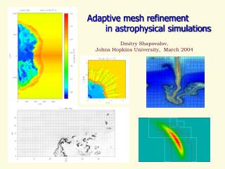
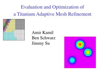
AMR Illustration • Adaptive meshes provide resolution where we need it • Several AMR Frameworks: CHOMBO, GrACE, SAMRAI, PARAMESH • CHOMBO, developed at LBNL, is the framework for enabling AMR • Prior experience with AMR using 8-wave upwinding + vector potential formulation on single fluid resistive MHD magnetic reconnection.
Adaptive Mesh Refinement with Chombo • Chombo is a collection of C++ libraries for implementing block-structured adaptive mesh refinement (AMR) finite difference calculations (http://www.seesar.lbl.gov/ANAG/chombo) • (Chombo is an AMR developer’s toolkit) • Mixed language model • C++ for higher-level data structures • FORTRAN for regular single grid calculations • C++ abstractions map to high-level mathematical description of AMR algorithm components • Reusable components. Component design based on mathematical abstractions to classes • Based on public-domain standards • MPI, HDF5 • Chombovis: visualization package based on VTK, HDF5 • Layered hierarchical properly nested meshes • Adaptivity in both space and time
Chombo Layered Design • Chombo layers correspond to different levels of functionality in the AMR algorithm space • Layer 1: basic data layout • Multidimensional arrays and set calculus • data on unions of rectangles mapped onto distributed memory • Layer 2: operators that couple different levels • conservative prolongation and restriction • averaging between AMR levels • interpolation of boundary conditions at coarse-fine interfaces • refluxing to maintain conservation at coarse-fine interfaces • Layer 3: implementation of multilevel control structures • Berger-Oliger time stepping • multigrid iteration • Layer 4: complete PDE solvers • Godunov methods for gas dynamics • Ideal and single-fluid resistive MHD • elliptic AMR solvers
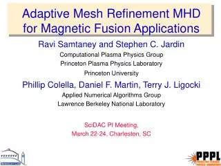
Results for S=104Parallel Run on NERSC IBM SP (4 nodes=64 processors, 5 AMR levels) Stage 1Middle islanddecays Stage 2Reconnection Stage 3Decay Y-component of B Z-component of B
Unsplit + Projection AMR Implementation • Implemented the Unsplit method using CHOMBO • Solenoidal B is achieved via projection, solving the elliptic equation r2=r¢ B • Solved on each level (union of rectangular meshes) • Coarser level provides Dirichlet boundary condition for • Requires O(h3) interpolation of coarser mesh on boundary of fine level • Solved using Multigrid on each level with a “bottom smoother” (conjugate gradient solver) when mesh cannot be coarsened • Physical boundary conditions are Neumann d/dn=0 • Multigrid convergence is sensitive to block size • Flux corrections at coarse-fine boundaries to maintain conservation • A consequence of this step: r¢ B=0 is violated on coarse meshes in cells adjacent to fine meshes. • Code is parallel • Second order accurate in space and time
Code verification – Plane wave propagation • A plane wave is initialized oblique to the meshInitial conditions for l-th characteristic waveW(x) = W0(x) + exp(i k¢ x) r_l • Plane wave chosen to correspond to Alfven velocity or fast magnetosonic sound speed • Low (=0.01) • Poisson solve converged in 8 iterations to a max residual of 10-14 • 3D Wave example
Code verification – Weak rotor problem with B field P with u field • Ideal MHD simulation of the “Rotor” problem (Balsara and Spicer, J. Comput. Phys. , Vol 149, 1999) • Independent code exists for cross verification (R. Crockett, Astrophysics, UC Berkeley) Poisson solver convergence history Conservation
Code verification – Weak rotor problem Conservation Poisson solver convergence history Pressure with B field lines
Conclusion and Future Work • A 3D conservative solenoidal B AMR code was developed • Preliminary verification test conducted • Plane wave tests • Rotor problem • More tests are underway in 2D and 3D • Future work • Addition of resistive and viscous terms • two-fluid MHD with Hall effect • 2D magnetic reconnection • Implicit treatment of fast wave • 3D magnetic reconnection