Download
1 / 17
170 likes | 283 Views
Performing Sensitivity Analysis for Ecological Models. Michael Mikucki Colorado State University 21 November 2009. Stage Structured Ecological Models. Discrete Time: Iterated Maps Previous Talk by Reid Thornton Life cycles grouped in states Transitioning between states: probabilities

E N D
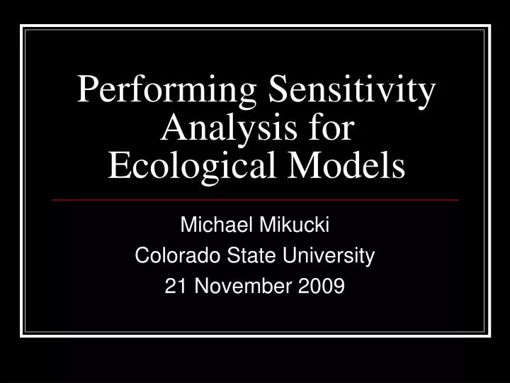
Performing Sensitivity Analysis for Ecological Models Michael Mikucki Colorado State University 21 November 2009
Stage Structured Ecological Models • Discrete Time: Iterated Maps • Previous Talk by Reid Thornton • Life cycles grouped in states • Transitioning between states: probabilities • Continuous Time: Differential Equations
Sensitivity Analysis • What is sensitivity? • States x1, x2, …, xi • Parameters p1, p2, …, pj • Initial Conditions x10, x20, …, xi0(treated as pj+1, …, pj+i) • Relative change in state with respect to a parameter • Interpretation • What are the benefits? • Data Collection • Management Strategies
Linear Sensitivity Calculations • Linear maps for ecological systems • xt+1 = Axt • xt is vector of states evaluated at time t • A is the transition matrix defining the system • Sensitivity of state xi with respect to parameter pj = dxi/dpj (at time t) • dxt+1/dp= (dA/dp)xt + A(dxt/dp) • Easy to calculate
Adding Nonlinearity (Caswell 2009) • 2 states • x1 – Juveniles • x2 – Adults • 4 parameters • f – adult fertility • σ1 – juvenile survival • σ2 – adult survival • γ – maturation probability • xt+1 = Axt where • Suppose σ1 depends on states • A depends on p and x dA/dp = (∂A/∂x)(dx/dp) + ∂A/∂p Caswell: Perturbation Analysis of Nonlinear Models (2009)
Adding Nonlinearity (Caswell 2009) Caswell: Perturbation Analysis of Nonlinear Models (2009)
Adding Nonlinearity (Caswell 2009) • Found ∂A/∂p and ∂A/∂x • Given initial values for f, γ, σ, σ2, we can iterate dx/dp in time dxt+1/dp= (dA/dp)xt + A(dxt/dp) = [(∂A/∂p) + (∂A/∂xt)(dxt/dp)] xt + A(dxt/dp) • Most difficult nonlinear sensitivity analysis to date • Increasingly difficult with more complicated models Caswell: Perturbation Analysis of Nonlinear Models (2009)
Form of Nonlinear Model • Caswell Example form • x(p,t+1) = A(x(p,t),p)*x(p,t) • Sensitivity of Caswell Example form • dx(t+1)/dp= [(∂A/∂p) + (∂A/∂xt)(dxt/dp)] xt + A(dxt/dp) • Treat as x(p,t+1) = g(x(p,t),p)) • dx(t+1)/dp = (∂g/∂x)(dx/dp) + ∂g/∂p
Caswell Example Rewritten • Want form x(t+1,p) = g(x(t,p),p) • dx(t+1)/dp = (∂g/∂x)(dx/dp) + ∂g/∂p • f • f
The Need for a Computerized System • Pine Model by R. Thornton • Nonlinear form • 12 states, 29 parameters= 348 derivatives • Longest derivative required 3,241 characters (no spaces) • Total of 97,846 characters (no spaces) • Automated differentiation
Graphical User Interface (GUI) • Direct Implementation • Model Equations • Parameters • Initial conditions • Number of Iterations • Indirect Implementation • Create own Maple code to input the above information • General outline provided • Press “Create Matlab files using Maple” button
GUI Technology • Creates MATLAB files using Maple • Automatic differentiation • Maple: ∂g/∂x, ∂g/∂p • MATLAB executes files by iterating dx/dp over time • Requires MATLAB 7.8.0 (R2009a), Maple 13, and “Maple toolbox for MATLAB”
Sensitivity Manipulation • Amount of plots (IPlot) • Want only specific states (IList) • Want only specific parameters (KList) • Want sensitivities at specific iterations • Want linear combination of solutions • Example: Sum/difference of 2 classes • QOI = < ψ, x > • d(QOI)/dp = < ψ, dx/dp >
Implementation of the GUI • Input Quantity of Interest Information • Iplot, IList, KList • Ψ Vector, QOI Times • Press the “Execute Matlab files” button
Continuous-time Sensitivity • ODE extension • x(t+1) = g(x(t,p),p) • dx/dt = g(x(t,p),p) Let z = dx/dp dz/dt = d/dt (dx/dp) = d/dp (dx/dt) **sensitivity of dx/dt = d/dp (g(x(t,p),p)) = (∂g/∂x)(dx/dp) + (∂g/∂p) = (∂g/∂x)z + ∂g/∂p • Numerical Error in dz/dt evaluation • Can do sensitivity analysis for continuous nonlinear models • SIR, cellular processes, Hodgkin Huxley, electrical circuits
Conclusions • Sensitivity analysis is crucial for ecological models • Discrete or continuous models • Need for automated differentiation (GUI) • Complicated models • Edits to the model • Extensions of the GUI lead to further research • Numerical error in continuous model analysis • Adjoint techniques in solving data
Acknowledgements Simon Tavener, Mike Antolin Colorado State University Funded in part by National Science Foundation Anna Schoettle United States Forest Service