Download
1 / 63
630 likes | 799 Views
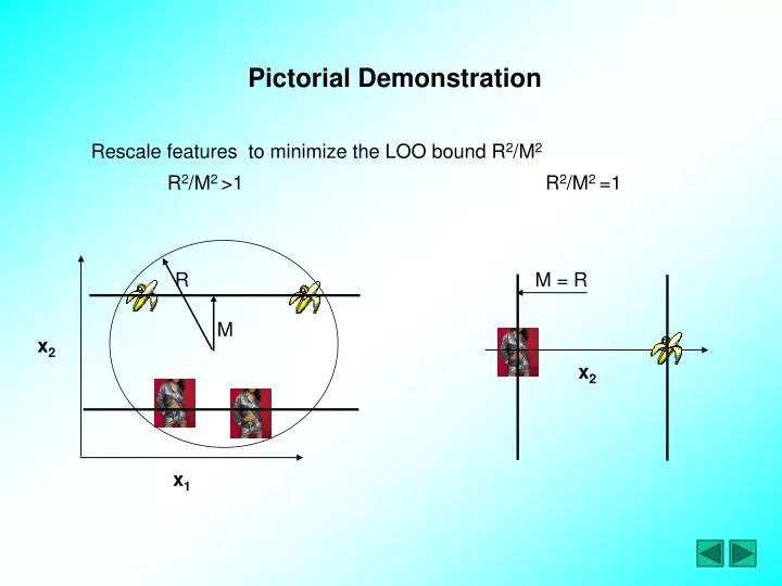
R 2 /M 2 = 1. R 2 /M 2 > 1. R. M = R. M. x 2. x 2. x 1. Pictorial Demonstration. Rescale features to minimize the LOO bound R 2 /M 2. SVM Functional. To the SVM classifier we add an extra scaling parameters for feature selection:.

E N D
R2/M2 =1 R2/M2 >1 R M = R M x2 x2 x1 Pictorial Demonstration Rescale features to minimize the LOO bound R2/M2
SVM Functional To the SVM classifier we add an extra scaling parameters for feature selection: where the parameters , b are computed by maximizing the the following functional, which is equivalent to maximizing the margin:
Toy Data Linear problem with 6 relevant dimensions of 202 Nonlinear problem with 2 relevant dimensions of 52
Face Detection On the CMU testset consisting of 479 faces and 57,000,000 non-faces we compare ROC curves obtained for different number of selected features. We see that using more than 60 features does not help.
p-val = 0.00039 p-val = 0.0015 Outcome Classification Error rates ignore temporal information such as when a patient dies. Survival analysis takes temporal information into account. The Kaplan-Meier survival plots and statistics for the above predictions show significance. Lymphoma Medulloblastoma
Part4 Clustering Algorithms Hierarchical Clustering
Step 1: Transform genes * experiments matrix into genes * genes distance matrix Step 2: Cluster genes based on distance matrix and draw a dendrogram until single node remains Hierarchical clustering
Hierarchical clustering (continued) To transform the genes*exp matrix into genes*genes matrix, use a gene similarity metric. (Eisen et al. 1998 PNAS 95:14863-14868) Exactly same as Pearsons correlation except the underline Where Gi equal the (log-transformed) primary data forgene G in condition i. For any two genes X and Y observed overa series of N conditions. Goffsetis set to 0, corresponding to fluorescence ratio of 1.0
Hierarchical clustering (continued) Pearsons correlation example What if genome expression is clustered based on negative correlation?
3 4 5 1 2 Hierarchical clustering (continued)
Part5 Clustering Algorithms k-means Clustering
K-means clustering This method differs from the hierarchical clustering in many ways. In particular, - There is no hierarchy, the data are partitioned. You will be presented only with the final cluster membership for each case. - There is no role for the dendrogram in k-means clustering. - You must supply the number of clusters (k) into which the data are to be grouped.
K-means clustering(continued) Step 1: Transform n (genes) * m (experiments) matrix into n(genes) * n(genes) distance matrix Step 2: Cluster genes based on a k-means clustering algorithm
K-means clustering(continued) To transform the n*m matrix into n*n matrix, use a similarity (distance) metric. (Tavazoie et al. Nature Genetics. 1999 Jul;22(3):281-5) Euclidean distance Where any two genes X and Y observed overa series of M conditions.
1 2 2 1 3 4 1 2 K-means clustering(continued)
K-means clustering algorithm Step 1: Suppose distance of genes expression patterns are positioned on a two dimensional space based a distance matrix Step 2: The first cluster center(red) is chosen randomly and then subsequent centers are by finding the data point farthest from the centers already chosen. In this example, k=3.
K-means clustering algorithm(continued) Step 3: Each point is assigned to the cluster associated with the closest representative center Step 4: Minimizes the within-cluster sum of squared distances from the cluster mean by moving the centroid (star points), that is computing a new cluster representative
K-means clustering algorithm(continued) Step 5: Repeat step 3 and 4 with a new representative Run step 3, 4 and 5 until no further changes occur.
Part6 Clustering Algorithms Principal Component Analysis
Principal component analysis (PCA) PCA is a variable reduction procedure. It is useful when you have obtained data on a large number of variables, and believe that there is some redundancy in those variables.
PCA (continued) - Items 1-4 are collapsed into a single new variable that reflects the employees’ satisfaction with supervision, and items 5-7 are collapsed into a single new variable that reflects satisfaction with pay. - General form for the formula to compute scores on the first component C1 = b11(X1) + b12(X2) + ……. b1p(Xp) where C1 = the subject’s score on principal component 1 b1p = the regression coefficient(or weight) for observed variable p, as used in creating principal component 1 Xp = the subject’s score on observed variable p.
PCA (continued) For example, you could determine each subject’s score on principal component 1 (satisfaction with supervision) and principal component 2 (satisfaction with pay ) by C1 = .44(X1) + .40(X2) + .47(X3) + .32(X4) + .02 (X5) + .01 (X6) + .03(X7) C2 = .01(X1) + .04(X2) + .02(X3) + .02(X4) + .48(X5) + .31 (X6) + .39(X7) These weights can be calculated using special type of equation called an eigenequation.
PCA (continued) (Alter et al., PNAS, 2000, 97(18) 10101-10106)
Part7 Clustering Algorithms Self-Organizing Maps
Clustering Goals • Find natural classes in the data • Identify new classes / gene correlations • Refine existing taxonomies • Support biological analysis / discovery • Different Methods • Hierarchical clustering, SOM's, etc
Self organizing maps (SOM) - A data visualization technique invented by Professor Teuvo Kohonen which reduce the dimensions of data through the use of self-organizing neural networks. - A method for producing ordered low-dimensional representations of an input data space. - Typically such input data is complex and high-dimensional with data elements being related to each other in a nonlinear fashion.
SOM (continued) - Cerebral cortex of the brain is arranged as a two-dimensional plane of neurons and spatial mappings are used to model complex data structures. - Topological relationships in external stimuli are preserved and complex multi-dimensional data can be represented in a lower (usually two) dimensional space.
SOM (continued) (Tamayo et al., 1999 PNAS 96:2907-2912) -One chooses a geometry of "nodes"for example, a3 × 2 grid. - The nodes are mapped into k-dimensional space, initiallyat random, and then iteratively adjusted. - Each iterationinvolves randomly selecting a data point P and moving the nodesin the direction of P.
SOM (continued) - The closest node NP is moved the most,whereas other nodes are moved by smaller amounts depending ontheir distance from NP in the initial geometry. - In this fashion,neighboring points in the initial geometry tend to be mapped tonearby points in k-dimensional space. The process continues for20,000-50,000 iterations.
SOM (continued) Yeast Cell Cycle SOM - The 828 genes that passed the variation filter were grouped into 30 clusters.
SOM analysis of data of yeast gene expression during diauxic shift [2]. Data were analyzed by a prototype of GenePoint software • a: Genes with a similar expression profile are clustered in the same neuron of a 16 x 16 matrix SOM and genes with closely related profiles are in neighboring neurons. Neurons contain between 10 and 49 genes • b: Magnification of four neurons similarly colored in a. The bar graph in each neuron displays the average expression of genes within the neuron at 2-h intervals during the diauxic shift • c: SOM modified with Sammon's mapping algorithm. The distance between two neurons corresponds to the difference in gene expression pattern between two neurons and the circle size to the number of genes included in the neuron. Neurons marked in green, yellow (upper left corner), red and blue are similarly colored in a and b
Result of SOM clustering of Dictyostelium expression data with a 6 x 4 structure of centroids. A 6 x 4 = 24 clusters is the minimum number of centroids needed to resolve the three clusters revealed by percolation clustering (encircled, from top to bottom: down-regulated genes, early upregulated genes, and late upregulated genes). The remaining 21 clusters are formed by forceful partitioning of the remaining non-informative noisy data. Similarity of expression within these 21 clusters is random, and is biologically meaningless.
SOM clustering • SOM - self organizing maps • Preprocessing • filter away genes with insufficient biological variation • normalize gene expression (across samples) to mean 0, st. dev 1, for each gene separately. • Run SOM for many iterations • Plot the results
SOM results Large grid 10x10 3 cells