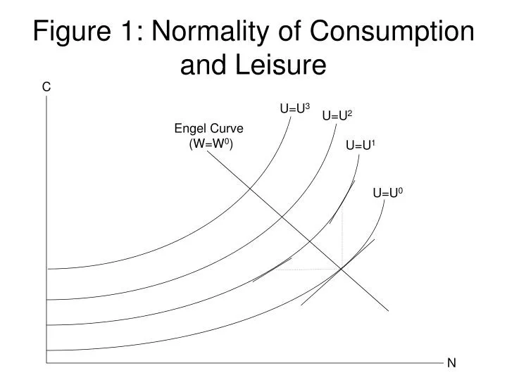
Figure 1: Normality of Consumption and Leisure

Figure 1: Normality of Consumption and Leisure C U=U3 U=U2 Engel Curve (W=W0) U=U1 U=U0 N

Figure 2: Long-Run Preferences and Technology Diagram (The Effect of an Increase in G) LMELR (W=W*) C MBLR (MBLR)´ C* C*´ N N* N*΄ -G -G’

Figure 3: A Higher W* Raises LMELR (the Engel Curve for W*) U=U3 (LMELR)´ (W=W*´) U=U2 U=U1 LMELR (W=W*) U=U0 N

Figure 4: Effect of an Increase in Z On Long-Run Equilibrium C (LMELR)´ LMELR (MBLR)´ MBLR C*´ C* N N*΄ N* -G

Figure 5:Utility-Accumulation Possibility Frontier U slope= -λ slope= -λ’ ´ dK/dt

Figure 6: The Factor Price Possibility Frontier R low K/(ZN) slope= -N/K high K/(ZN) FPPF(Z) W

Figure 7: Labor Supply and Demand W Ns(λ) + Nd(K,Z) + + N

Figure 8: An Increase in Labor Supply W Ns(λ) Ns(λ’) Nd(K,Z) N

Figure 9: An Increase in K Raises Labor Demand W Ns(λ) Nd(K’,Z) Nd(K,Z) N

Figure 10: An Increase in K Causes a Movement Along the FPPF R K/(ZN) low K/(ZN) high FPPF(Z) W

Figure 11: An Improvement in Technology Shifts the FPPF Out R FPPF(Z) FPPF(Z’) W

Figure 12: Phase Diagram • λ • λ=0 saddle path • λ0 λ* • K=0 K K0 K*

Figure 13: DGE Effects of a Permanent Increase in G λ • λ=0 λ0 λ*new λ*old • K=0 (new) • K=0 (old) K K*old K*new

Figure 14: DGE Effects of a Permanent Increase in Z(Wealth Effect Dominates Rental Rate Effect) λ • • λ=0 (old) λ=0 (new) λ*old λ0 λ*new • K=0 (old) • K=0 (new) K K*old K*new

Figure 15: DGE Effects of a Permanent Increase in Z(Rental Rate Effect Dominates Wealth Effect) λ • • λ=0 (old) λ=0 (new) λ0 λ*old λ*new • K=0 (old) • K=0 (new) K K*old K*new

Figure 16: DGE Effects of a Permanent Increase in Z(Equal and Opposite Wealth and Rental Rate Effects) λ • • λ=0 (old) λ=0 (new) λ*old λ*new • K=0 (old) • K=0 (new) k K*old K*new

Figure 1: Normality of Consumption and Leisure