Download
1 / 21
210 likes | 303 Views
Stability Analysis of Pedestrian Flow in 2D OV Model with Asymmetric Interaction. Tian Huan-huan Xue Yu. August 13, 2013. Outline. Review the 1D OV Model Review the 2D OV Model The 2D OV Model with the asymmetric interaction Linear stability analysis Conclusions. 1. The 1D OV Model.

E N D
Stability Analysis of Pedestrian Flow in 2D OV Model with Asymmetric Interaction Tian Huan-huan Xue Yu August 13, 2013
Outline • Review the 1D OV Model • Review the 2D OV Model • The 2D OV Model with the asymmetric interaction • Linear stability analysis • Conclusions
1. The 1D OV Model • ------the coordinate of the nth vehicle • -----the acceleration • -----------the driver’s sensitivity • -----the optimal velocity (OV) function [1] BANDO M, HASEBE K, NAKAYAMA A, et al. Phys. Rev. E, 1995, 51:1035–1042.
2. The 2D OV Model (TOVM) • -----the position of jth pedestrian • -----the desired velocity • -----the interaction between pedestrians [2] SUGIYAMA Y, NAKAYAMA A, HASEBE K. PED’01, 155-160 [3] NAKAYAMA A, HASEBE K, SUGIYAMA Y. Physical Review E, 2005, 71:036121.
The strength of the interaction is determined by the distance (between jth and kth pedestrians) and the angle (between and ); • indicated that the pedestrian is more sensitive to pedestrians in front than those behind.
The interaction is • The first derivative of the function is centered on the inflectant point; That’s to say, the process of the acceleration and deceleration is symmetrical in the pedestrian flow, so the interaction between pedestrians is symmetrical. • In reality, the response to the acceleration and deceleration is different. Especially in a high-density situation, in order to avoid collision and pushing, pedestrians are willing to slow down, which is similar with drivers’ behavior.
The homogeneous solution of equation (1) is is a constant vector ; is a constant velocity . Consider a small perturbation as follows:
(2) The linearized equations of equation(1) are (3) where
Suppose that the small wave propagates at the angle with the x axis.
The 2D wave is classified into two types of modes: longitudinal mode and transverse mode. • The longitudinal mode The linearized equations (2) and (3) are
The transverse mode The linearized equations (2) and (3) are
4. Conclusions • The asymmetrical interaction between pedestrians is considered in the 2D OV model. • The stability of homogenous flow is investigated with linear stability analysis. • The phase diagram is obtained. • The critical curve of longitudinal mode move leftward along r-axis and the regions below the curves of longitudinal mode becomes smaller. The critical curve of transverse mode move rightward along r-axis.
The phase diagram is obtained. There are six regions above the critical curves in the new model. The region A in the original model is divided into two regions (A and E) in new model, the region C in the original model is divided into two regions (C and F) in new model.