Download
1 / 37
370 likes | 497 Views
Temporal Framework for Monitoring Rangeland Sustainability: A Discussion By Robert A. Washington-Allen Research & Development Staff Environmental Sciences Division Oak Ridge National Laboratory P.O. Box 2008, MS 6407 Oak Ridge, TN 37831-6407 E-mail: washingtonra@ornl.gov.

E N D
Temporal Framework for Monitoring Rangeland Sustainability: A Discussion By Robert A. Washington-Allen Research & Development Staff Environmental Sciences Division Oak Ridge National Laboratory P.O. Box 2008, MS 6407 Oak Ridge, TN 37831-6407 E-mail: washingtonra@ornl.gov
What is a temporal framework? What is monitoring? What is condition? What is trend? What is a standard or reference? When do you begin monitoring? How do you relate indicators? What about causality?
Monitoring (Applied Ecology) Objectives 1. Detect change in the extent and distribution of indicators. 2. Assess rangeland condition and trend. 3. Suggest causality 4. Assess the risk of future crises. O’Neill, R.V., C. Hunsaker, and D. Levine. 1994. Monitoring challenges and innovative ideas. Proc. Int. Sym. Ecological Indicators.
Monitoring Challenges: • Landscapes are middle-number systems. • When indicators are re-measured some values will have changed: • Does the change indicate a trend or normal fluctuations (historical variation)? • Reliable evidence of trends require monitoring over long periods. • For rangelands, current literature suggests 15 to 20 years if you wish to capture periodic climatic events (e.g., ENSO, La Nina, and PDO) or fire return intervals.
Illustration of Ecological Statics and Dynamics From: Turner, M.G., R.H. Gardner, and R.V. O’Neill. 2001. Landscape ecology in theory and practice. Springer-Verlag, New York, N.Y.
100000 Land Systems Catena Size of ranch 10000 domain of pasture Ecological sites/land units production Foraging range of cattle Foraging range of sheep 1000 domain of landscape degradation 100 sheet erosion Landsat MSS pixel size Spatial scale (m) Landsat Landsat TM pixel size 10 1 water erosion features Ground individual plants 0.10 1 10 100 1000 10000 100000 Temporal; Scale (days) Estimated frequency Of wilfires in Sagebrush steppe Soil regeneration Lifetime of most perennial plants Estimated frequency of severe droughts Rainfall event Landsat overpass Vegetation greenup The relationship of space and time to observable phenomena. The paradigm suggests the scales at which phenomena will act, provides an investigator with the constraints on experimental design, and suggests the tools required to detect phenomena of interest (adapted from Graetz 1987).
A principle of Ecosystem science and Landscape Ecology is that before any ecosystem or landscape can be studied it must be bounded in space and time. Grain and Extent must be explicitly stated.
Grain constrains the spatial and temporal scale of observation. The coarsest resolution defines the studies grain.
NALC MSS 58m MSS 79m
Condition: A one-time measure of change in an indicator relative to a standard. Trend: A temporal measure of change in an indicator. The magnitude of a trend can be measured using a significant regression coefficient of the indicator versus time. Standard: The reference that provides the basis for comparison that allows determination of a significant change. Reference conditions can be subjective or objective: the average (mean, mode, or median), maximum, or minimum conditions.
Ways to Monitor Levels of Control Differ Experimental: Laboratory Lab-Field Field Retrospective Studies: Opportunistic, but usually lack controls and replications. Studies of longer temporal scales depend upon conditions which may no longer exist, i.e., suffer from lack of analogues for contemporary comparisons. Computer Simulations Also Note: Regional scale studies: Usually lack controls and replication, consequently not amenable to traditional statistical designs.
However, the systematic determination of a statistically significant trend (or an ecologically significant trend)may take years to determine. O’Neill, R.V., C. Hunsaker, and D. Levine. 1994. Monitoring challenges and innovative ideas. Proc. Int. Sym. Ecological Indicators.
Time series analyses set the analytical domain for trend data. This includes: Data transformations: Log Moving average Differencing Analystics: Autocorrelation Autoregression Non-linear time series Spectral/Fourier Cross correlation Intervention
How do these metrics relate to each other and through time? The example above can be viewed either as 3 different sites being compared or 1 site moving through its multivariate envelope.
disturbance start alternative state malleability end amplitude threshold Historical Variation CHRONIC DISTURBANCE ACUTE DISTURBANCE hysteresis attribute attribute time time Adapted from Westman (1988), Hosten (1995).
Legend Mean Variance Grand Mean Centroid Cluster 0.1 Increasing Greenness 0.09 0.08 0.07 0.06 Increasing Heterogeneity of Greenness 95 0.05 SAVI Variance 0.04 84 96 74 82 0.03 80 89 97 76 72 85 79 75 73 86 0.02 87 91 81 90 88 0.01 0 0.2 0.25 0.3 0.35 0.4 0.45 0.5 0.55 SAVI Mean The dry season soil-adjusted vegetation index (SAVI) statistical phase portrait for the sagebrush steppe portion of Deseret Land & Livestock Company ranch from 1972 to 1997.
1972 1973 1974 1975 1976 1979 1980 1981 1982 1984 1985 1986 1987 1988 1989 1990 1991 1992 Dry Season 1994 1995 1996 1997 The dry season time series of soil-adjusted vegetation index (SAVI) images of the sagebrush steppe portion of Deseret Land & Livestock Company ranch from 1972 to 1997.
T2 T1,T6 Shrubland (B) Native Grassland (G) T4 Threshold T5 T3 T3 T4,T6 Threshold T3,T5 > 60 % Shrub Dense Shrubland (D) Introduced Grasses (F) T1: fire, T2: grazing, T3: heavy grazing, T4: cultural inputs, T5: drought, T6: wetter than average years sparse grass/ bare soil dense grass/ bare soil denser grass/ bare soil shrub grass/ bare soil Spatial hypothesis of temporal change in landscape pattern and structure in relation to climate change, grazing, and fire. The spatial map was adapted from West and Young (2000).
1980 1988 1995 1972 1981 1989 1996 1973 1974 1982 1990 1997 1975 1985 1991 1976 1986 1992 1979 1987 1994 The growth form and land cover (bare ground) time series of thematic maps of the sagebrush steppe dominated portion of Deseret Land & Livestock Co. Ranch. The maps were derived from dry season Landsat MSS and TM satellite imagery from 1972 to 1997.
Grass Cover Shrub Cover % Grass Cover % Shrub Cover Contagion Time The predicted response of growth-form composition and contagion to relatively high frequency of droughts and high grazing intensity. These predictions are the results of 200-year computer simulation model developed by Li and Reynolds (1998). The rate of change in contagion and physiognomy happened rapidly and abruptly relative to low and moderate frequencies of drought and grazing pressure.
1.00 0.90 Mean 1987 - 1997 0.80 0.70 0.60 Grand Mean 0.50 Shrub/Grass Cover Ratio 0.40 Mean 1972 - 1987 0.30 0.20 0.10 0.00 1970 1974 1976 1978 1988 2000 1972 1980 1982 1984 1986 1990 1992 1994 1996 1998 Dry Season Year
r2 = 0.35 p = 0.0015 n = 26 1.0 .5 0.0 -.5 -1.0 1 3 5 7 9 11 13 15 17 19 21 Lag Year
Monitoring can suggest, but it can seldom demonstrate causality. • Monitoring can only hope to show correlations. • O’Neill, R.V., C. Hunsaker, and D. Levine. 1994. Monitoring challenges and innovative ideas. Proc. Int. Sym. Ecological Indicators.
0.55 0.5 0.45 0.4 0.35 0.3 0.25 0.2 wet dry wet dry wet dry wet dry wet dry wet dry wet dry wet dry wet dry wet dry wet dry dry wet dry Garff, Freed, & Robinson 1972-1975 J. Hotung 1975 -1983 LDS Farm Management Group 1983 - 1998 0.60 0.60 0.60 0.58 0.58 0.58 Y= 0.0005x2 - 0.01x + 0.41 r2 = 0.07 p = 0.58 n = 16 0.56 Y= 0.0005x2 - 0.01x + 0.46 r2 = 0.40 p = 0.003 n = 31 Y= 0.02x + 0.29 r2 = 0.32 p = 0.18 n = 7 0.56 0.56 0.54 0.54 0.54 0.52 0.52 0.52 0.50 0.50 0.50 0.48 0.48 0.48 0.46 0.46 0.46 0.44 Mean SAVI 0.44 0.44 0.42 Mean SAVI 0.42 Mean SAVI 0.42 0.40 0.40 0.40 0.38 0.38 0.38 0.36 0.36 0.36 0.34 0.34 0.34 0.32 0.32 0.32 0.30 0.30 0.30 0.28 0.28 0.28 0.26 0.26 Continuous Grazing Rotational Grazing Short Duration Grazing 0.26 0.24 0.24 0.24 0.22 0.22 0.22 0.20 0.20 0.20 1973 1974 1974 1975 1975 1972 1973 1975 1975 1976 1976 1977 1977 1978 1978 1979 1979 1980 1980 1981 1981 1982 1982 1983 1983 1992 1983 1983 1984 1984 1985 1985 1986 1986 1987 1987 1988 1988 1989 1989 1990 1990 1991 1991 1992 1993 1993 1994 1994 1995 1995 1996 1996 1997 1997 1998 Season-Year Season-Year Season-Year 1953-1975 1975-1983 1983-1998 Mean SAVI Mean Management Period Cubic Fit (cubic fit, r2 = 0.29, p = .003) wet dry wet dry wet dry wet wet dry wet dry wet wet dry dry wet wet dry dry wet dry wet dry dry wet dry wet 72 73 74 75 76 77 78 79 80 81 82 83 84 85 86 87 88 89 90 91 92 93 94 95 96 97 98 Season-Year The seasonal wet and dry soil-adjusted vegetation index (SAVI) time series for the sagebrush steppe portion of Deseret Land & Livestock Company ranch from 1972 to 1998. The 3 management regimes and the best fit for each regime and the entire time series are curvilinear regression line are delineated. Missing years were replaced by linear interpolation.
Dust Bowl 1950s 87 to 89 Mean interannual Palmer Drought Severity Index (PDSI) from 1895 to 1996 for the Northern Mountains Climatic Region 5. PDSI values from -4 or less indicate extreme drought and from 4 or greater extreme wet periods (Alley 1984). These data were acquired from the Utah Climate Center.
1980 1981 1982 1983 1984 1985 1992 1993 1994 1995 1996 1997 1986 1987 1988 1989 1990 1991 The apparent spatial distribution of livestock from 1980 to 1997 at the paddock-level on Deseret Land & Livestock Company Ranch.
Drought in the last 2000 years , North Dakota 1200 http://www.ngdc.noaa.gov/paleo/drought/drght_2000years.html Laird, K. R., S. C. Fritz, K. A. Maasch, and B. F. Cumming. 1996. Greater drought intensity and frequency before A.D. 1200 in the Northern Great Plains, U.S.A. Nature 384:552-554.
Hughes, M. K. and L. J. Graumlich. 1996. Climatic variations and forcing mechanisms of the last 2000 years. Volume 141. Multi-millenial dendroclimatic studies from the western United States. NATO ASI Series, pp. 109-124.
Landscapes are middle-number systems. Farming is still a high-risk venture.
1996 1994 1994 1994 1992 Fires (yellow polygons) detected on the Deseret Land & Livestock Company Ranch from 1992 to 1996 using Landsat Multispectral Scanner and Thematic Mapper (TM) satellite imagery. An 1994 Indian Resource Satellite (IRS) scene, which has been merged to a false-color TM scene, and a polygon coverage of the grazing paddocks serve as the backdrop.
Number of Patches Mean Patch Size Contagion r = 0.99 p = 0.09 n = 3 r = -0.32 p = 0.79 n = 3 r = -0.99931 p = 0.02 n = 3 Mean Nearest Neighbor Nearest Neighbor SDE Contagion r = -0.96 p = 0.17 n = 3 r = -0.92 p = 0.26 n = 3 r = -0.99 p = 0.07 n = 3 Retrospective inference of the relationship of landscape-scale metrics with extent and perimeter of fire on the eastern portion of Deseret Land & Livestock Co. Ranch from 1972 to 1997 using linear regression. For the relationship of fire perimeter with landscape-scale metrics, only the significant correlation of with contagion ( p ≤ 0.10) is shown.
16000 0.60 Grand Mean = 7034 AU 1891 to 1903 = 7548 AU 1915 to 1951 = 10633 AU 14000 1967 to 1998 = 4444 AU 0.50 12000 0.40 10000 Animal Unit (AU) 8000 0.30 Mean SAVI 6000 0.20 4000 0.10 2000 0 0.00 1891 1895 1899 1903 1907 1911 1915 1919 1923 1927 1931 1935 1939 1943 1947 1951 1955 1959 1963 1967 1971 1974 1976 1978 1980 1982 1984 1986 1988 1990 1992 1994 1996 1998 Year The time series of seasonal soil-adjusted vegetation index (SAVI) from 1972 to 1998 (line plot) in relation to the time series of animal units (combined sheep and cattle, bar chart) from 1891 to 1998.
0.60 0.50 0.40 0.30 0.20 0.10 0.00 wet dry wet dry wet dry wet dry wet dry wet dry wet dry wet dry wet dry wet dry wet dry dry wet dry wet dry wet dry wet dry wet dry wet dry Year 72 73 74 75 76 77 78 79 80 81 82 83 84 85 86 87 88 89 90 91 92 93 94 95 96 97 8 6 4 2 PDSI 0 Mean SAVI -2 -4 -6 -8 wet dry wet dry wet dry wet dry wet dry wet dry wet dry wet dry Season Mean SAVI PDSI 5 per. Mov. Avg. (PDSI) A comparison between the 1972 to 1997 time series of the seasonal month of image acquisition Palmer Drought Severity Index (PDSI), the 5-year moving average of PDSI, and the seasonal soil-adjusted vegetation index (SAVI) of the Rich County-sagebrush steppe portion of Deseret Land & Livestock Company ranch.
1100 90 1050 80 1000 70 MPS 950 y = 64x + 48 60 R 2 = 0.89 p = 0.00004 900 n = 10 50 Number of Patches Mean Patch Size (Ha) 850 NP y = -793x + 1052 40 R 2 = 0.81 800 p =0.0004 n = 10 30 750 20 700 10 650 600 0 0.000 0.100 0.200 0.300 0.400 0.500 0.600 Bulk Stocking Density (AU/Ha) Land NP MPS Linear (Land NP) Linear (MPS)
Clumped Deposition Grassland E High Production A B F Erosion Fragmented C D Low Production El Niño Shrubland Soil Moisture La Niña Grazing Pressure Modified to 3-D from Holmgren et al. (2001)
How long do you monitor? Temp. Years before present (1000) Vostok Ice Core: The Vostok temperature record indicates that the earth has been colder than present for most of the past 250,000 years, including many ice ages . J. Jouzel, C. Waelbroeck, B. Malaiz, M. Bender, J. R. Petit, N. I. Barkov, J.M. Barnola, T. King, V. M. Kotlyakov, V. Lipenkov, C. Lorius, D. Raynaud, C.Ritz and T. Sowers, Climatic interpretation of the recently extended Vostok ice records, Clim.Dyn., In press
Longer time scales: Robert Frost Planning Horizon Fire and Ice