Basic Statistics and Monte-Carlo Method -2

1. Applied Statistical Mechanics Lecture Note - 10 Basic Statistics and Monte-Carlo Method -2 고려대학교 화공생명공학과 강정원

2. Table of Contents • General Monte Carlo Method • Variance Reduction Techniques • Metropolis Monte Carlo Simulation

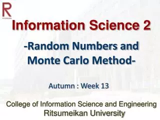
3. 1.1 Introduction • Monte Carlo Method • Any method that uses random numbers • Random sampling the population • Application • Science and engineering • Management and finance • For given subject, various techniques and error analysis will be presented • Subject : evaluation of definite integral

4. 1.1 Introduction • Monte Carlo method can be used to compute integral of any dimension d (d-fold integrals) • Error comparison of d-fold integrals • Simpson’s rule,… • Monte Carlo method • Monte Carlo method WINS, when d >> 3 purely statistical, not rely on the dimension !

5. 1.2 Hit-or-Miss Method • Evaluation of a definite integral • Probability that a random point reside inside the area • N : Total number of points • N’ : points that reside inside the region h X X X X X X O O O O O O O a b

6. 1.2 Hit-or-Miss Method Start Set N : large integer N’ = 0 h X X X X X Choose a point x in [a,b] X Loop N times O O O O O Choose a point y in [0,h] O O a b if [x,y] reside inside then N’ = N’+1 I = (b-a) h (N’/N) End

7. 1.2 Hit-or-Miss Method • Error Analysis of the Hit-or-Miss Method • It is important to know how accurate the result of simulations are • The rule of 3s’s • Identifying Random Variable • From central mean theorem , is normal variable in the limit of large N

8. 1.2 Hit-or-Miss Method • Sample Mean : estimation of actual mean value (m) • Accuracy of simulation  the most probable error

9. 1.2 Hit-or-Miss Method • Estimation of error • We do not know exact value of s , m • We can also estimate the variance and the mean value from samples …

10. 1.2 Hit-or-Miss Method • For present problem (evaluation of integral) exact answer (I) is known  estimation of error is,

11. 1.3 Sample Mean Method • r(x) is a continuous function in x and has a mean value ;

12. 1.3 Sample Mean Method • Error Analysis of Sample Mean Method • Identifying random variable • Variance

13. 1.3 Sample Mean Method • If we know the exact answer,

14. 1.3 Sample Mean Method Start Set N : large integer s1 = 0, s2 = 0 xn = (b-a) un + a Loop N times yn = r(xn) s1 = s1 + yn , s2 = s2 + yn2 Estimate mean m’=s1/N Estimate variance V’ = s2/N – m’2 End

15. QUIZ • Compare the error for the integral using HM and SM method

16. Example : Comparison of HM and SM • Evaluate the integral

17. Example : Comparison of HM and SM • Comparison of error • No of evaluation having the same error SM method has 36 % less error than HM SM method is more than twice faster than HM

18. 2.1 Variance Reduction Technique - Introduction • Monte Carlo Method and Sampling Distribution • Monte Carlo Method : Take values from random sample • From central limit theorem, • 3s rule • Most probable error • Important characteristics

19. 2.1 Variance Reduction Technique - Introduction • Reducing error • *100 samples reduces the error order of 10 • Reducing variance  Variance Reduction Technique • The value of variance is closely related to how samples are taken • Unbiased sampling • Biased sampling • More points are taken in important parts of the population

20. 2.2 Motivation of Variance Reduction Technique • If we are using sample-mean Monte Carlo Method • Variance depends very much on the behavior of r(x) • r(x) varies little  variance is small • r(x) = const  variance=0 • Evaluation of a integral • Near minimum points  contribute less to the summation • Near maximum points  contribute more to the summation • More points are sampled near the peak ”importance sampling strategy”

21. 2.3 Variance Reduction using Rejection Technique • Variance Reduction for Hit-or-Miss method • In the domain [a,b] choose a comparison function • Points are generated on the area under w(x) function • Random variable that follows distribution w(x) w(x) r(x) X X X X X O O O O O O O a b

22. 2.3 Variance Reduction using Rejection Technique • Points lying above r(x) is rejected w(x) r(x) X X X X X O O O O O O O a b

23. 2.3 Variance Reduction using Rejection Technique • Error Analysis Hit or Miss method Error reduction

24. 2.3 Variance Reduction using Rejection Technique Start Set N : large integer w(x) r(x) X X N’ = 0 X X X O Generate u1, x= W-1(Au1) O Loop N times O O O O O Generate u2, y=u2 w(x) a b If y<= f(x) accept value N’ = N’+1 Else : reject value I = (b-a) h (N’/N) End

25. 2.4 Importance Sampling Method • Basic idea • Put more points near maximum • Put less points near minimum • F(x) : transformation function (or weight function_

26. 2.4 Importance Sampling Method if we choose f(x) = cr(x) ,then variance will be small The magnitude of error depends on the choice of f(x)

27. 2.4 Importance Sampling Method • Estimate of error

28. 2.4 Importance Sampling Method Start Set N : large integer s1 = 0 , s2 = 0 Generate xnaccording to f(x) Loop N times gn = r (xn) / f ( xn) Addgn to s1 Add gn to s2 I ‘ =s1/N , V’=s2/N-I’2 End

29. 3. Metropolis Monte Carlo Method and Importance Sampling • Average of a property in Canonical Ensemble Probability

30. 3. Metropolis Monte Carlo Method and Importance Sampling • Create nirandom points in a volume riN such that • Problem : How we can generate ni random points according to We cannot use inversion method Use Markov chain with Metropolis algorithm

31. 3. Metropolis Monte Carlo Method and Importance Sampling • Markov chain :Sequence of stochastic trials satisfies few some conditions • Stochastic process that has no memory • Selection of the next state only depends on current state, and not on prior state • Process is fully defined by a set of transition probabilitiespij pij= probability of selecting state j next, given that presently in state i. Transition-probability matrix Pcollects all pij

32. Markov Chain • Notation • Outcome • Transition matrix • Example • Reliability of a computer • if it is running 60 % of running correctly on the next day • if it is down it has 80 % of down on the next day

33. Markov Chain limiting behavior always converges to a certain value independent of initial condition Stochastic matrix : sum of the probability should be 1 • Features • Every state can be eventually reached from another state • The resulting behavior follows a certain probability