Download
1 / 50
500 likes | 656 Views
debris disc modelling. Philippe Thébault Paris Observatory/Stockholm Observatory. Disc modelling: going from there…. …to there…. …and there. Outline. I . Observational data: the need for modelling II . Size and spatial distributions of debris discs III . Collisional avalanches

E N D
debris disc modelling Philippe Thébault Paris Observatory/Stockholm Observatory
Outline • I. Observational data: the need for modelling • II. Size and spatial distributions of debris discs • III. Collisional avalanches • IV. Outer edges of debris discs • V. Vertical structure of debris discs (work in progress)
what is a debris disc? • it is not a protoplanetary disc • Lagrange et al.(2000): • Mdisc<<0.01 M* • Ldisc/L*<<1 • Dust and gas dynamics decoupled (Mgas<10Mdust) • Dust lifetime < System’s age (« debris ») • debris discs are made from collisionally eroding leftovers from the planet-formation process
relative timescales: collisions are the dominant process! Example: β-Pic (Artymowicz, 1997)
protoplanetary discs around YSOs Young (<107yrs) and massive (~100M) discs, with Mgas/Mdust~100
« protoplanetary » discs Debris discs Greaves (2005)
Discoveries of debris discs, the IR trilogy: IRAS/ISO/Spitzer IRAS (ESA, 1983): all sky survey. Resolution~0.5’-2’. First IR-excess detection: Vega (“vega-type” stars). ~170 IR-excess detections => ~15% of stars with debris discs ISO (ESA, 1996): pointed telescope. Resolution~1.5”-90”. 22 new detections. ~17% of stars with discs. Spectral type dependancy: A:40%, F:9%, G:19%, K:8%. Spitzer (NASA, 2003): pointed telescope, currently operating. Resolution~1”-10”. Truckload of new results coming out.
Imaging of debris discs: visible/near IR b-Pictoris (1984)
0.5µm 0.5µm 1-2µm 10-20µm 850µm β-Pictoris: multi wavelength imaging
Circumstellar disc observations: wavelength vs radius probed Circumstellar discs have been studied at all wavelengths from optical to cm Different wavelengths probe different locations in the disc; e.g., thermal emission from an optically thin disc, assuming black body grains: Tdust = 278.3 L*0.25/r0.5 peak = 2898m/T = 10.4r0.5/L*0.25 rprobed = 0.012L*0.5 AU NIR=0.1AU, MIR=1AU, FIR=30AU, SUB=1000AU (though smaller as not observed at peak)
What do we se? DUST (<1cm) • Total flux = photometry • One wavelength shows disk is there • Two wavelengths determines dust temperature • Model fitting with multiple wavelengths (Spectral Energy Distribution) • Composition = spectroscopy • Can be used like multiple photometry • Also detects gas and compositional features • Structure = imaging • Give radial structure directly and detects asymmetries • But rare as high resolution and stellar suppression required Scattered light: UV, visible,near-IR Thermal emission:mid-IR,far-IR,mm
Deriving dust masses: sub-mm/mm photometry • Sub-mm/mm observations are the best way of deriving dust mass: • unaffected by uncertainties in Tdust • discs are optically thin so most of the mass is seen • larger grains contain most of the mass • little contribution to flux from stellar photosphere • The basic equation is: • Mdust = Fd2/[B(T)] • where d is distance, = 1.5Q/(D) 0(0/) is the mass opacity and a value of 0=0.17m2/kg is often used for 0=850m with =1
what we see • Dust ~ [µm,mm] • Gas (sometimes) what we’d like to know about • pebbles, rocks, planetesimals, asteroids, comets.… • Planets
Numerical Modelling, why? • Observations only give partial (size, radial location) and model dependent information SED • Most of the mass (r>1cm) remains undetectable SB profile
Numerical Modelling, what for? • What are discs made of? • Size Distribution • Total mass • “hidden” bigger parent bodies (>1cm) • Long term evolution, lifetime AND OR • What is going on? • Explain the Observed Spatial Structures • Presence of Planets?
II. Collisional Evolution models • Derive accurate size & spatial distributions for the whole visible grain populations • Characterize the invisible population of eroding parent bodies • Understand what is going on: dynamical state, mass loss rate, presence of transitory events, etc….
Size Distributions derived from observations are model dependent… (Li & Greenberg 1998)
what we see ...and restricted to a narrow size range collisional cascade ~radiation pressure cutoff unseen parent bodies size distribution ??? ~observational limit
? doing it the lazy way: the drr3.5dr distribution Theoretical collisional-equilibrium law dN r-3.5dr What we don’t see What we see
many reasons why the dNr3.5dr distribution just doesn’t work • assumes infinite size distribution • wrong: rmin due to radiation pressure rmaxbecause finite mass • assumes scale-independent collisional processes • wrong: response to impacts varies with size (strength regime for small targets, grav.regime for big ones) • neglects the specific dynamics of small grains • wrong: radiation places high-β on eccentric orbits
Size Distribution/Evolution:Statistical “Particle in a box” Models • Principle • Dust grains distributed in Size Bins (and possibly spatial/velocity bins) • “Collision” rates between all size-bins • Each bini-binj interaction produces a distribution of binl<max(i,j) fragments • Approximations/Simplifications • No (or poor) dynamical Evolution • Poor spatial resolution
statistical collisional evolution code • « Particle in a box » Principle • divide the population in size bins • evolution Equ.: • Collision Outcome prescription (lab.experiments)
a5 a4 da a3 a2 a1 a(1), e(1) High e orbits of grains close to the RPR limit multi-annulus collisional code (Thebault&Augereau, 2007) • takes into account • Collisions (fragmentation, cratering, re-accretion) • simplified dynamics • Radiation pressure effects • Extended Disc: 10-120AU • Size range: 1μm – 50km (!)
evolution of an extended debris disc size distribution evolution (Thebault&Augerau, 2007)
(2) overabundance due to the lack of smaller potential impacotrs (1) Lack of grains< RPR (3) Depletion due to the overabundance in (2) (4) Overdensity due to lack of (3), etc… cutoff size RPR the ”wavy” size distribution
collision rates the ”magical” tcol=(Ωτ)-1formula can also be *very* wrong
why should we care? / Main Conclusions • Wavyness is a robust feature • Overdensity of ~2rcutoff grains • Depletion of 10rcut<r<50rcut grains • Optical depth dominated by a narrow range rcut<r<2rcut • visible dust radial distribution ≠ parent bodies distribution • (flatter) (steeper by a factor ~a) Be careful when reconstructing ”asteroid belts”
Main Conclusions (2) • this has consequences on data anlysis from Spitzer/Herschel...
III. Collisional avalanches Grigorieva, Thebault&Artymowicz 2007 Could clumpy or spiral structures be explained by transient violent collisional events?
collisional avalanches: combined statistical and dynamical code Collisionnal cascade after large planetesimal/cometary breakup
IV. Outer edges of debris discs: how sharp is sharp?
Outer edges: ”natural” collisional evolution of a narrow ring left to itself a-3.5 slope (Thébault & Wu, 2008)
processes at play • Collisions in the ”birth ring” produce high-β grains on high-e orbits • Steady state: 0.2<β<0.4 grains dominate in the aring<a<4rring region
the ”universal” a-3.5profile low mass disc high mass disc
”extreme” case with SB profile steeper than a-3.5 dynamically ”cold” system: e=2i < 0.01 main problem: how likely is it? high-β grains production is unefficient (low v among parent bodies) while high-β grains destruction is still very efficient (high v among small grains) => Depletion of β>0.1 grains
in short ”natural” outer edge profile ”natural” if highly anisotropic scattering ”natural” only if e<0.01...otherwise, need for ”something” else to act
V. Vertical structure of debris discs (work in progress) • Very few discs are resolved in z • the H/a ratio is our only reliable information on the disc’s dynamical state... if equipartition: H/a ~ 2<i>~<e> ~ <dV>/VKep ex: H/a=0.1 => <dV>~ 450m/s => Vesc(RBIG) ~ 450m/s => RBIG~500km • ...or is it? => Radiation Pressure on small grains!
a numerical experiment Q: how do mutual collisions redistribute orbital elements for a population of grains affected by Radiation Pressure? • ”bouncing balls” code • ~20000 test particles • Size distribution: dnrdr • Size range: 0.04<β<0.4 • Inelastic collisions Thébault & Brahic (1995)