Download

1 / 43
430 likes | 614 Views
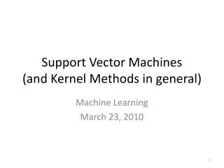
Data Mining and Mathematical Programming Workshop Centre de Recherches Mathématiques Universit é de Montr é al, Qu é bec October 10-13, 2006. Nonlinear Knowledge in Kernel Machines. Olvi Mangasarian UW Madison & UCSD La Jolla Edward Wild UW Madison. Objectives.

E N D
Data Mining and Mathematical Programming Workshop Centre de Recherches Mathématiques Université de Montréal, Québec October 10-13, 2006 Nonlinear Knowledge in Kernel Machines Olvi Mangasarian UW Madison & UCSD La Jolla Edward Wild UW Madison
Objectives • Primary objective: Incorporate prior knowledge over completely arbitrary sets into: • function approximation, and • classification • without transforming (kernelizing) the knowledge • Secondary objective: Achieve transparency of the prior knowledge for practical applications
h1(x) · 0 g(x) · 0 h2(x) · 0 Graphical Example of Knowledge Incorporation + + + + + + + + K(x0, B0)u = • Similar approach for approximation
Outline • Kernels in classification and function approximation • Incorporation of prior knowledge • Previous approaches: require transformation of knowledge • New approach does not require any transformation of knowledge • Knowledge given over completely arbitrary sets • Fundamental tool used • Theorem of the alternative for convex functions • Experimental results • Four synthetic examples and two examples related to breast cancer prognosis • Classifiers and approximations with prior knowledge more accurate than those without prior knowledge
Theorem of the Alternative for Convex Functions:Generalization of the Farkas Theorem • Farkas: For A2 Rk£ n, b2 Rn, exactly one of the following must hold: • I. Ax 0, b0x > 0 has solution x2Rn, ,or • II. A0 v=b, v 0, has solution v2Rk . • Let h:½Rn!Rk, :!R, convex set, h and convexon , andh(x)<0 for some x2. Then, exactly one of the following must hold: • I. h(x) 0, (x) < 0 has a solution x, or • II. vRk, v 0: v0h(x)+(x) 0 x. • To get II of Farkas: • v 0, v0Ax- b0x 0 8 x2Rn ,v 0, A0 v-b=0.
Classification and Function Approximation • Given a set of m points in n-dimensional real space Rn with corresponding labels • Labels in {+1, -1} for classification problems • Labels in R for approximation problems • Points are represented by rows of a matrix A2Rm£n • Corresponding labels or function values are given by a vector y • Classification: y2 {+1, -1}m • Approximation: y Rm • Find a function f(Ai) = yibased on the given data points Ai • f : Rn ! {+1, -1} for classification • f : Rn! R for approximation
Classification and Function Approximation • Problem: utilizing only given data may result in a poor classifier or approximation • Points may be noisy • Sampling may be costly • Solution: use prior knowledge to improve the classifier or approximation
Adding Prior Knowledge • Standard approximation and classification: fit function at given data points without knowledge • Constrained approximation: satisfy inequalitiesat given points • Previous approaches (2001 FMS, 2003 FMS, and 2004 MSW ): satisfy linearinequalities over polyhedral regions • Proposed new approach: satisfy nonlinearinequalities over arbitrary regions without kernelizing (transforming) knowledge
Kernel Machines • Approximate f by a nonlinear kernel function K using parameters u 2Rk and in R • A kernel function is a nonlinear generalization of the scalar product • f(x) K(x0, B0)u - , x 2Rn, K:Rn£Rn£k!Rk • Gaussian K(x0, B0)i=-||x-Bi||2, i=1,…..,k • B 2Rk£nis a basis matrix • Usually, B = A2Rm£n = Input data matrix • In Reduced Support Vector Machines, B is a small subset of the rows of A • B may be any matrix with n columns
Kernel Machines • Introduce slack variable sto measure error in classification or approximation • Error s in kernel approximation of given data: • -sK(A, B0)u -e - ys, e is a vector of ones in Rm • Function approximation: f(x) K(x0,B0)u - • Error s in kernel classification of given data • K(A+, B0)u - e + s+¸e, s+¸ 0 • K(A- , B0)u - e - s- -e, s-¸ 0 • More succinctly, let: D = diag(y), the m£m matrix with diagonal y of § 1’s, then: • D(K(A, B0)u - e) + s¸ e, s¸0 • Classifier: f(x) sign(K(x0,B0)u -)
Kernel Machines in Approximation Kernel Machines in Approximation OR Classification • Trade off between solution complexity (||u||1) and data fitting (||s||1) • At solution • e0a = ||u||1 • e0s = ||s||1 OR
Incorporating Nonlinear Prior Knowledge: Previous Approaches • Cxdw0x- h0x + • Need to “kernelize” knowledge from input space to transformed (feature) space of kernel • Requires change of variable x = A0t, w = A0u • CA0t d u0AA0t - h0A0t+ • K(C, A0)tdu0K(A,A0)t - h0A0t+ • Use a linear theorem of the alternative in the tspace • Lost connection with original knowledge • Achieves good numerical results, but is not readily interpretable in the original space
Nonlinear Prior Knowledge in Function Approximation: New Approach • Start with arbitrary nonlinear knowledge implication • g(x) 0K(x0, B0)u - h(x), 8x2 ½ Rn • g, h are arbitrary functions on • g:! Rk, h:! R • Linear in v, u, 9v¸ 0: v0g(x) + K(x0, B0)u - - h(x) ¸ 0 8x2
Theorem of the Alternative for Convex Functions • Assume that g(x), K(x0, B0)u - , -h(x) are convex functions of x, that is convex and 9x2 : g(x)<0. Then either: • I. g(x) 0, K(x0, B0)u - - h(x) < 0 has a solution x,or • II. vRk, v 0: K(x0, B0)u - - h(x) + v0g(x) 0 x • But never both. • If we can find v 0: K(x0, B0)u - - h(x) + v0g(x) 0 x, then by above theorem • g(x) 0, K(x0, B0)u - - h(x) < 0 hasno solution x or equivalently: • g(x) 0 K(x0, B0)u - h(x), 8x2
Proof • I II (Not needed for present application) • Follows from a fundamental theorem of Fan-Glicksburg-Hoffman for convex functions [1957] and the existence of an x2 such that g(x) <0. • I II (Requires no assumptions on g, h, K, or uwhatsoever) • Suppose not. That is, there exists x2, v 2Rk,, v¸ 0: • g(x) 0, K(x0, B0)u - - h(x) < 0, (I) • v 0, v0g(x) +K(x0, B0)u - - h(x) 0 , 8 x 2 (II) • Then we have the contradiction: • 0 > v0g(x) +K(x0, B0)u - - h(x) 0 · 0 < 0
Incorporating Prior Knowledge • Linear semi-infinite program: infinite number of constraints • Discretize: finite linear program • g(xi) · 0 )K(xi0, B0)u - ¸h(xi), i = 1, …, k • Slacks allow knowledge to be satisfied inexactly • Add term to objective function to drive slacks to zero
Numerical Experience: Approximation • Evaluate on three datasets • Two synthetic datasets • Wisconsin Prognostic Breast Cancer Database (WPBC) • 194 patients £ 2 histogical features • tumor size & number of metastasized lymph nodes • Compare approximation with prior knowledge to approximation without prior knowledge • Prior knowledge leads to an improved accuracy • General prior knowledge used cannot be handled exactly by previous work (MSW 2004) • No kernelization needed on knowledge set
Two-Dimensional Hyperboloid • f(x1, x2) = x1x2
Two-Dimensional Hyperboloid x2 • Given exact values only at 11 points along line x1 = x2 • At x12 {-5, …, 5} x1
Two-Dimensional Hyperboloid Approximation without Prior Knowledge
Two-Dimensional Hyperboloid • Add prior (inexact) knowledge: • x1x2 1 f(x1, x2) x1x2 • Nonlinear term x1x2 can not be handled exactly by any previous approaches • Discretization used only 11 points along the line x1 = -x2, x1 {-5, -4, …, 4, 5}
Two-Dimensional Tower Function (Misleading)Data • Given 400 points on the grid [-4, 4] [-4, 4] • Values are min{g(x), 2}, where g(x) is the exact tower function
Two-Dimensional Tower Function Approximation withoutPrior Knowledge
Two-Dimensional Tower FunctionPrior Knowledge • Add prior knowledge: • (x1, x2) [-4, 4] [-4, 4] f(x) = g(x) • Prior knowledge is the exact function value. • Enforced at 2500 points on the grid [-4, 4] [-4, 4] through above implication • Principal objective of prior knowledge here is to overcome poor given data
Two-Dimensional Tower Function Approximation with Prior Knowledge
Breast Cancer Application:Predicting Lymph Node Metastasis as a Function of Tumor Size • Number of metastasized lymph nodes is an important prognostic indicator for breast cancer recurrence • Determined by surgery in addition to the removal of the tumor • Optional procedure especially if tumor size is small • Wisconsin Prognostic Breast Cancer (WPBC) data • Lymph node metastasis and tumor size for 194 patients • Task: predict the number of metastasized lymph nodes given tumor size alone
Predicting Lymph Node Metastasis • Split data into two portions • Past data: 20% used to find prior knowledge • Present data: 80% used to evaluate performance • Past data simulates prior knowledge obtained from an expert
Prior Knowledge for Lymph Node Metastasis as a Function of Tumor Size • Generate prior knowledge by fitting past data: • h(x) := K(x0, B0)u - • B is the matrix of the past data points • Use density estimation to decide where to enforce knowledge • p(x) is the empirical density of the past data • Prior knowledge utilized on approximating function f(x): • Number of metastasized lymph nodes is greater than the predicted value on past data, with tolerance of 0.01 • p(x) 0.1 f(x) ¸h(x) - 0.01
Predicting Lymph Node Metastasis: Results • RMSE: root-mean-squared-error • LOO: leave-one-out error • Improvement due to knowledge: 14.9%
Incorporating Prior Knowledge in Classification (Very Similar) • Implication for positive region • g(x) 0K(x0, B0)u - , 8x2 ½ Rn • K(x0, B0)u - - + v0g(x) ¸ 0, v ¸ 0, 8x2 • Similar implication for negative regions • Add discretized constraints to linear program
Numerical Experience: Classification • Evaluate on three datasets • Two synthetic datasets • Wisconsin Prognostic Breast Cancer Database • Compare classifier with prior knowledge to one without prior knowledge • Prior knowledge leads to an improved accuracy • General prior knowledge used cannot be handled exactly by previous work (FMS 2001, FMS 2003) • No kernelization needed on knowledge set
100 100 Prior Knowledge for 16-Point Checkerboard Classifier Checkerboard Classifier With Knowledge Using 16 Center Points Checkerboard Classifier Without Knowledge Using 16 Center Points
Prior Knowledge Function for Spiral Spiral Classifier With Knowledge Spiral Classifier Without KnowledgeBased on 100 Labeled Points Note the many incorrectly classified +’s White ) + Gray ) • Labels given only at 100 correctly classified circled points Prior knowledge imposed at 291 points in each region No misclassified points
Predicting Breast Cancer Recurrence Within 24 Months • Wisconsin Prognostic Breast Cancer (WPBC) dataset • 155 patients monitored for recurrence within 24 months • 30 cytological features • 2 histological features: number of metastasized lymph nodes and tumor size • Predict whether or not a patient remains cancer free after 24 months • 82% of patients remain disease free • 86% accuracy (Bennett, 1992) best previously attained • Prior knowledge allows us to incorporate additional information to improve accuracy
Generating WPBC Prior Knowledge • Gray regions indicate areas where g(x) · 0 • Simulate oncological surgeon’s advice about recurrence • Recur within 24 months Knowledge imposed at dataset points inside given regions Number of Metastasized Lymph Nodes • Cancer free within 24 months • Recur • Cancer free Tumor Size in Centimeters
WPBC Results 49.7 % improvement due to knowledge 35.7 % improvement over best previous predictor
Conclusion • General nonlinear prior knowledge incorporated into kernel classification and approximation • Implemented as linear inequalities in a linear programming problem • Knowledge appears transparently • Demonstrated effectiveness • Four synthetic examples • Two real world problems from breast cancer prognosis • Future work • Prior knowledge with more general implications • User-friendly interface for knowledge specification • Generate prior knowledge for real-world datasets
Website Links to Talk & Papers • http://www.cs.wisc.edu/~olvi • http://www.cs.wisc.edu/~wildt