Download
1 / 42
420 likes | 558 Views
Challenges for finite volume models. Haroldo F. de Campos Velho haroldo@lac.inpe.br http://www.lac.inpe.br/~haroldo. Outline. Few words on finite volume (FV) approach Patankar’s FV approach for CFD The driven cavity flow Investigations Mixed grids Fractal cavity

E N D
Challenges for finite volume models Haroldo F. de Campos Velho haroldo@lac.inpe.br http://www.lac.inpe.br/~haroldo
Outline • Few words on finite volume (FV) approach • Patankar’s FV approach for CFD • The driven cavity flow • Investigations • Mixed grids • Fractal cavity • Step back: some FV discretizations
Few words on finite volume • We can consider some strategies for solving PDE • Domain decomposition • Boundary decomposition • Spectral methods • Finite volume is a domain decomposition method • Partition the computational domain into control volumes (which are not necessarily the cells of the mesh) • Discretise the integral formulation of the conservation laws over each control volume (Gauss divergence theorem). • Solve the resulting set of algebraic equations or update the values of the dependent variables.
FV: integral form • A key issue: integral form of conservation law: • applying the Gauss divergence theorem (there are some advantages for considering conservative form instead of non-conservative one)
Source terms • It is difficult to maintain the balance of the form • applying standard finite volume approach: Gauss theorem can not be applied to the source term.
An application: incompressible fluid • We starting from the fluid dynamics formulation • Initial and boundary conditions
Some remarks on incompressible fluid • Incompressible fluid is consider a simpler version of the N-S equation. • Is it the above statement true? • Yes and no: Yes: there are less equations to be solved. No: Who is the integration factor?
Integration factor • Simple ODE: • the integration factor is: , therefore
Integration factor • Matrix ODE: • If P-1 exists:
Integration factor • Incompressible fluid: who is the pressure? • Is there an integration factor? • Clearly: M-1 does not exist. Mathematical tools: • Drazin generalized inverse (ODE) - after discretization • Application of a type singular semi-group (PDE).
Integrating incompressible fluid • Deriving a Poisson equation for pressure • with Neumann boundary conditions
FV: discrete version 1. The flux terms are discretised by where is the numerical flux.
FV: discrete version 1. For 2D flow:
FV: discrete version 1. For 2D flow:
FV: discrete version For 2D flow (pressure: white; velocities: blue): Patankar staggered grid control volume (red) Grid cell node
FV: discrete version – a question: Looking at the figure: Why should not we use a simple triangular control volume (black), instead of red one? And then, the bad dream started …
What would we want? • We were trying to study a fluid flow inside of a fractal domain. • The first idea is to use unstructured grids • We were also interested to investigate a mixed grid (combining structured grid + unstructured grid). • Why is someone interested in mixed grid? • Obvious reason: improve computational performance.
Driven cavity flow • This is easier fluid dynamical problem that it must be solved by numerical process.
Studing fractal cavity flow • Koch curve generator: • Two pre-fractals:
Studing fractal cavity flow • Fractal cavity + finite volume decomposition
FV: unstructured grids baricenter
FV: unstructured grids • Grid-(a): work! • Grid-(b): doesn’t work • Grid-(c): doesn’t work • Grid-(d): doesn’t work Why?
Answering the question • S. Abdallah (J. Comput. Phys., 70, 1987) has shown that structured grids obey the compatibility equation. • How about the unstrutured grids?
Answering the question • The compatibility equation: it is an identity in fluid dynamics. • The solution for the Poisson eqution for pressure exists if the compatibility condition is verified:
Discrete compatibility equation • Using the discrete pressure Poisson equation • Assuming (Sa edge size):
Fractal cavities properties • Attractors for fractal cavities: (a) standard cavity (b) fractal cavity
Co-localized approaches • Someone should be surprised with the results, where cell-center and cell-vertex did not work. • Beause, some authors have used cell-center and cell-vertex, and such procedures presented good results. • What’s wrong?
Co-localized approaches • Actually, nothing is wrong. • However, the evil is in details: • Co-localized variables and cell-center: - Frink’s approach (AIAA, 1994): he use a different interpolation scheme. - Marthur-Marthy (Num. Heat Transf., 1997): they uses a different scheme to compute the gradient. • Velocities located at vertex, and pressure at barycenter: - Thomadakis-Leschziner (Num. Methods Fluids, 1996): The control volume is computed with union of barycenter, we used median-dual scheme.
Spectral schemes x Finite volume • Finite volume approaches can be used in a more complex domain (geometry). • Recent results are indicating that for high resolution, spectral schemes have a bigger computational effort than finite volume. • Which is the future for the spectral schemes? • Maybe, it depends on the type of computing used.
Spectral schemes x Finite volume • Transforms (FFT/Legendre) could be implemented in a hybrid computing: hardware and software for processing. • Hybrid computing: FPGA, GPU.
Spectral schemes x Finite volume • Enhancing the computing: appering the first optical processors. • Optical processors (FPGA): (a) Lenslet (Mar/2003) (b) Intel (Feb/2006)
Final remarks • Structured grid the compatibility equation is always verified. • Compatibility condition can be used to select a type of unstrutured grid. • Nothing is neutral in numerical approximation. • Remember: the evil is in details.
Preliminar Analysis • Smallest cube: L = 120 h-1 Mpc • 1.7107 2.2106 particules runing time ~ 60 h • redshift computed • z = 10.0, 1.0, 0.1 e 0.0 • Edge effect • L z <n> • 239.5 Mpc todos 1.22 • 120 Mpc 10.0 1.23 • 120 Mpc 1.0 1.27 • 120 Mpc 0.1 1.29 • 120 Mpc 0.0 1.30
Percolation (FoF) • Percolation radius • Rperc = b <R> f = n / <n> 2/ b3 • Mass scales:M(Np) M(M) class • 1 71010 small and galaxies • LMC 2 1010 M • 2-50 21011—31012 “regular” galaxies • Via-Láctea 7 1011 M • M87 3 1012 M • 50-15k 31012 —11015 groups or clusters • Grupo Local 4 1012 M • Coma 1 1015 M • > 15k > 11015 superaclusters • SA Local 2 1015 M • Rperc b f Np • Gal. 0.1 0.11 1500 2-50 VL 10 part. (R=100-150 kpc) • Cluster 0.184 0.2 250 50-15000 Gr. Local 55 part. • SA 1.25 1.15 2 > 15000 SA Local 30000 part.