Download
1 / 24
250 likes | 299 Views
Understand Discrete-Time Fourier Transform, its properties, spectrum of signals, polar and rectangular forms, and relationship to Discrete Fourier Transform. Learn about signal symmetry and examples of signal computations.

E N D
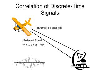
Ch.4 Fourier Analysis of Discrete-Time Signals Kamen and Heck
4.1 Discrete-Time Fourier Transform • X() = n=-, x[n] e -jn (Eq. 4.1) • Complex valued function of real variable , the frequency. • A sufficient condition for x[n] to have a DTFT in the ordinary sense is that x[n] be absolutely summable.
Example 4.1 Computation of the DTFT Consider x[n] = an, 0nq and 0 otherwise. The DTFT is X() = n=-, x[n] e -jn = n=0,q an e -jn = n=0,q (ae -j)n = [1 – (ae -j)q+1 ] / [1- (ae -j)] (where the closed form expression for a partial sum exponential is used—(Eq.4.5)
4.1 Discrete-Time Fourier Transform (cont.) • X() is a periodic function of with period 2. • Rectangular Form: X() = R() + jI(). R() = n=-, x[n] cos(n) I() = - n=-, x[n] sin(n) • Polar Form: X() = |X()| +exp[j X()]. • |X()| = SQRT[R2() + I2()]. • X()=tan-1[I()/ R()] when R() 0 • = + tan-1[I()/ R()] when R() < 0
Example 4.2 Rectangular and Polar Forms • Consider x[n] = an u(n). • This is similar to Ex. 4.1 except we have q. • Consider the DTFT from Ex. 4.1 but let q: • X() = lim q [1 – (ae -j)q+1 ] / [1- (ae -j)] • This limit exists for |a| < 1. • For this case, the DTFT exists in the ordinary sense. • X() = 1/ [1- (ae -j)] (Eq. 4.16) • The rectangular and polar forms are shown on pages 170-171.
4.1.1 Signals with Even or Odd Symmetry • Let x[n] be a real-valued discrete-time signal that is an even function (ie, x[n] = x[-n].) • The DTFT is X()= x[0] + n=1, 2x[n] cos(n) • Let x[n] be an odd function (ie,x[n]=-x[-n]) • The DTFT is X()= x[0] - n=1, j2x[n]sin(n)
Example 4.3 DTFT of Rectangular Pulse • Let p[n] = 1 for -q n q and 0 elsewhere. • The signal is even but it is easier to use 4.2. • P() = n=-q,q e -jn • =[ e jq – e -j(q+1) ] / [1- e -j ] • = sin[(q + 1/2) ]/[sin(/2)] • This is the discrete-time counterpart to the transform of the rectangular pulse (Ex. 3.9). • Figure 4.3 illustrates the DTFT.
4.1.2 Spectrum of a Discrete-Time Signal • For simplification, the discrete-time Fourier series is not discussed. • For a discrete time signal that is not a function of sinusoids the spectrum is a continuum of frequency components. • The frequency spectrum is made up of the amplitude spectrum and the phase spectrum. • The highest value of = .
Example 4.4 Decaying Exponential • Assume that x[n] = (.5)n u(n). • The signal is plotted in Fig. 4.1. • The spectrum is shown in Figure 4.2 • Note that most of the spectrum is in the lower frequencies.
Example 4.5 Signal with High-Frequency Components • Consider x[n] = (-.5)n u(n). • From Figure 4.4 we see that there should be higher frequency components in this signal. • From the result of Ex 4.2, the DTFT is: • X() = 1/ [1- (-.5e -j)] = 1/ [1 + .5e -j] • The amplitude and phase spectra are given by equations 4.25 and 4.26 and plotted in Figure 4.5.
4.1.3 Inverse DTFT • x[n] = 1/2 02 X() e jn d (Eq. 4.7)
4.1.4 Generalized DTFT • Example 4.6 DTFT of a Constant Signal • Let x[n] =1 for all n. • This signal does not have a DTFT in the ordinary sense—(Why?) • Figure 4.6 shows the generalized DTFT. • Discussion on page 176 illustrates that its inverse is the constant signal.
DTFT Transform Pairs and Properties • 4.1.5 Transform Pairs—Table 4.1 page 177. • Properties—Table 4.2 page 178. • No duality property, but there is a relationship between the inverse of the CTFT and the DTFT. • Result can be used to generate DTFT pairs from CTFT pairs—see Example 4.7.
4.2 Discrete Fourier Transform • Let x[n] be a discrete-time signal. • Let X() is the DTFT of x[n]. • Note: the DTFT is a continuous function of . • Let N be a positive integer, then the DFT of x[n] is: • Xk = n=0,N-1 x[n] e -j2kn/N , k=0,1,2,…N-1
4.2 The DFT (p.2) • In general, Xk is a function of the discrete integer k. • There are N values in the DFT of x[n]. • These values are complex numbers. • Polar form: Xk = |Xk| exp [jXk] • Rectangular form: Xk = Rk + jIk • See equations 4.36, 4.37. • MATLAB—program on page 180.
4.2 The DFT (p.3) • Example 4.8 Computation of the DFT • Finite sequence –page 181. • 4.2.1 Symmetry • Magnitude of the DFT is symmetric about N/2, for N even. • Phase angle of the DFT has odd symmetry about N/2 when N is even. • 4.2.2 Inverse DFT—see equation 4.40 and MATLAB program and Example 4.9 on page 183.
The DFT (p.4) • 4.2.3 Sinusoidal Form • The right hand side of the IDFT equation can be written as sinusoids. • See equation 4.45 and Example 4.10. • 4.2.4 Relationship to DTFT • If x[n] = 0 for n<0 and n N, the DFT Xk can be viewed as a freqeuency sample version of the DTFT. • Xk =X() =2k/N = X(2k/N ), k = 0,1,2,…,N-1
Example 4.11 DTFT and DFT of a Pulse • Consider p[n] from example 4.3. • Let x[n] be p[n-q]. • Figure 4.10 shows the amplitude spectrum for q=5. • Figure 4.11 shows the amplitude of the DFT for q=5 and N= 22. • Figure 4.12 shows the amplitude of the DFT for q=5 and N = 88.
4.4 FFT Algorithm • Consider the DFT and Inverse DFT: • Xk = Σn=0,1,…,N-1 x[n] e -j2kn/N k=0,1,…,N-1 • x[n]= (1/N ) Σk=0,…,N-1 Xk e j2kn/N, n=0,…,N-1 • How many multiplications are needed to compute the DFT? (N2) • The FFT algorithm requires N(log2N)/2 multiplications.
4.4 FFT Algorithm (p.2) • If N = 1024, • DFT requires 1,048,576 multiplications • FFT requires 5,120 multiplications • There are different variations of the FFT algorithm. • One uses “decimation-in-time”.
4.4 FFT (p.3) • Decimation-in-Time • Subdivide the time interval into intervals having a smaller number of points.
4.4 FFT (p.4) • Xk can be broken up into two parts. • First let exp(-j2/N) = WN • Then Xk = Σn=0,1,…,N-1 x[n]( WN )kn k=0,1,…,N-1 • Let N be an even integer: a[n]=x[2n] ; b[n]=x[2n + 1], for n = 0,…,N/2. • Let Ak = Σn=0,…,N/2-1a[n] (WN/2)kn, k=0,1,…N/2-1 • Let Bk = Σn=0,…,N/2-1b[n] (WN/2)kn, k=0,1,…N/2-1 • Then Xk = Ak + (WN)k Bk, k=0,1,…,N/2 -1 • And X(N/2)+k = Ak - (WN)k Bk, k=0,1,…,N/2 -1 • See page 197 for the verification.
4.4 FFT (p.5) • Note that the two parts are (N/2) DFTs. • This can continue until signals with only one nonzero value are obtained if N is a power of 2. • The process is graphically illustrated by Figure 4.21. • To have the outputs in the correct order, a process called bit reversing (see Table 4.3) is used.
4.4.1 Applications of the FFT Algorithm • Computation of the Fourier Transform • Convolution • Data Analysis • Extraction of a Sinusoidal Component Embedded in Noise • Analysis of Sunspot Data • Stock Price Analysis