Download
1 / 59
610 likes | 668 Views
Delve into the Sun's atmosphere, magnetic field, coronal heating, and solar wind dynamics. Learn about historical milestones, corona's temperature profiles, and solar emission processes.

E N D
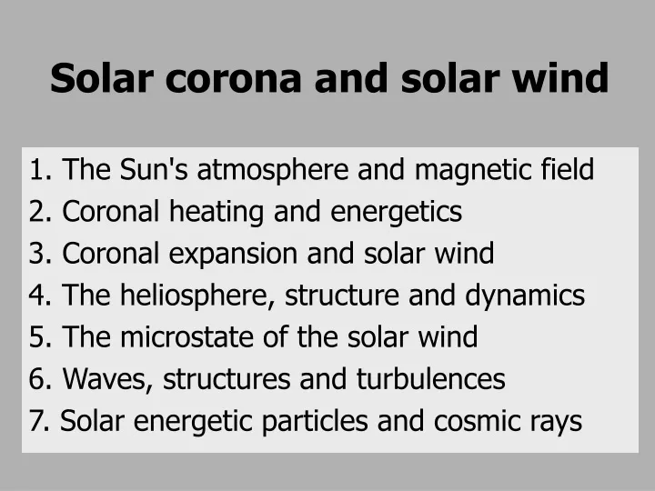
Solar corona and solar wind 1. The Sun's atmosphere and magnetic field 2. Coronal heating and energetics 3. Coronal expansion and solar wind 4. The heliosphere, structure and dynamics 5. The microstate of the solar wind 6. Waves, structures and turbulences 7. Solar energetic particles and cosmic rays
The Sun's atmosphere and magnetic field • The Sun's corona and magnetic field • EUV radiation of the corona • The magnetic network • Doppler spectroscopy in EUV • Small-scale dynamics and turbulence • Temperature profiles in the corona
Corona in late May 2002 1.3 MK EIT/SOHO Fe IX,X 17.1 nm SOHO EIT SOHO EIT Fe IX,X 17.1 nm Fe IX,X 17,1 nm Fe IX,X 17.1 nm
Some historical dates I • 1000 (BC) China: Correlations betwenn sunspots and aurora; geomagnetism is known and the magnetic needle • 500 (BC) Greece: Magnetism • 350 (BC) Theophrastus observes sunspots with naked eye • 1200 England: compass, Neekam -> navigation • 1600 W. Gilbert in England: „de magnete“ • 1850 F. Gauß in Germany: Earth magnetic field, mathematical analysis (multipole expansion) and measurements (10-5 precision); currents inside earth (dynamo) and in the atmosphere • 1814 Fraunhofer discovers hundreds of solar lines (prism) • 1843 Schwabe: Sunspot activity cycle (11 years) • 1860 Loomis: auroral oval ( 20o - 25o) • 1908 Hale: sunspots have strong magnetic fields
Some historical dates II • 1920 Existence of Earth ionosphere from radio waves (whistlers) • 1930 „Clouds“ of particles and magnetic fields from solar flares (broadband flashes of light) on the Sun • 1940 Edlén and Grotrian, coronal emission from highly ionised elements, temperature T > 1 MK • 1958 Explorer 1, Earth radiation belts (van Allen) • 1958 E. Parker: Solar wind as supersonic plasma flow • 1950 Leighton: 5-minute oscillations in photosphere • 1962 Mariner 2, Solar wind (in-situ) measurements • 1962/4 Explorer 12/OGO, Bow shock wave in front of the Earth magnetosphere • 1996 SOHO, comprehensive solar observations from space (near libration point at about 1Mkm)
The visible solar corona Eclipse 11.8.1999
Electron density in the corona • + Current sheet and streamer belt,closed • Polar coronal hole,openmagnetically Heliocentric distance / Rs Guhathakurta and Sittler, 1999, Ap.J., 523, 812 Skylab coronagraph/Ulysses in-situ
Corona and magnetic network 80000 K 1996 SOHO EIT He II 30.4 nm
Active regions near minimum 2 MK 1996 SOHO EIT Fe XV 28.4 nm
Corona and transition region 2000000 K 1.3 MK 2001 1300000 K SOHO EIT Fe IX,X 17.1 nm SOHO EIT Fe IX,X 17,1 nm Fe IX,X 17.1 nm
Active regions near maximum 1.6 MK 2001 SOHO EIT SOHO EIT Fe XII 19.5 nm
EUV line excitation processes • Collisional excitation of atom or ion, A, followed by a radiative decay: • A + e- --> A* + e- (ne > 108 cm-3) • A* --> A + hLine radiance: L ne2 • Resonant scattering (fluorescence): • A + h --> A* --> A + hLine radiance: L ne • Radiative recombination: • A+z + e- --> A+(z-1)* --> A+z-1 + h
Solar EUV emission spectrum Ly Spectral intensity/ mWm2sr-1Å-1 Curdt et al., A&A 375, 591, 2001 Wavelength / Å SOHO SUMER
Elementary radiation theory I Coronal model approximation: collisional excitation and radiative decay Ng(X+m) ne Cg,j = Nj Aj,g Cg,j [cm3s-1] collisional excitation rate Aj,g [s-1] atomic spontaneous emission coefficient ( 1010s-1) Emissivity (power per unit volume): P(g,j ) = Nj(X+m) Aj,g Ej,g [erg cm3 s-1] Eg,j = Ej - Eg photon energy Ng(X+m) number density of ground state of ion X+m
Elementary radiation theory II Occupation number density of level j of an ion (m-fold ionized atom) of the element X: Nj(X+m)/ne = Nj(X+m)/N(X+m) • N(X+m)/N(X) • N(X)/n(H) • n(H)/ne excitation levelionic fractionabundancen(H) [cm3] hydrogen Collisonal excitation rate (Maxwellian electrons): Ci,j 1/Te1/2 exp{ Ei,j /(kBTe) } Boltzmann factor
Oxygen ionization balance N like He like H like First ionization potential (FIP) I = 13.62 eV LTE -> N(X+m)/N(X) follows from Saha‘s equation; ~ exp(-I/kBTe) Shull and van Steenberg, ApJ. Suppl. 48, 95; 49, 351, 1982
Emission measure Emissivity in the line of ion X+m: P(g,j) = N(X+m)/N(X) N(X)/n(H) n(H)/ne Cg,jEg,j ne2 Contribution function (strongly peaked in Te): G(Te, g,j) = N(X+m)/N(X) Cg,j Emission measure: < EM > = V ne2 dV The emission measure depends on the amount of plasma (at temperature Te) emitting in the observed spectral line. Radiation power (line strength) < EM >
The Sun as a star: EUV spectrum Pagano et al., 2001
X-ray corona Yohkoh SXT 3-5 Million K
Loops near the solar limb CDS Loop Observations CDS 1998/3/23
Corona of the active sun 1998 EIT - LASCO C1/C2
Changing corona and solar wind 45 30 15 0 -15 -30 -45 North Heliolatitude / degree South LASCO/Ulysses McComas et al., 2000
Coronal magnetic field and density Dipolar, quadrupolar, current sheet contributions Polar field: B = 12 G Current sheet is a symmetric disc anchored at high latitudes ! LASCO C1/C2 images (SOHO) Banaszkiewicz et al., 1998; Schwenn et al., 1997
MHD model coronal magnetic field closed open „Elephants trunk“ coronal hole Linker et al., JGR, 104, 9809, 1999
The Sun‘ open magnetic field lines MHD model field during Ulysses crossing of ecliptic in early 1995 Mikic & Linker, 1999
Small magnetic flux tubes and photospheric granulation White: Flux tubes Scale 100 km 35 Mm x 40 Mm Magnetic regions (seen in G-band near 430 nm) between granules Scharmer, 1993
Changing coronal magnetic field minimum • Model extrapolation: • Potential field, B=0 • Force-free field, jxB=0 Solar cycle variation maximum Bravo et al., Solar Phys.,1998
The elusive coronal magnetic field Future: High-resolution imaging and spectroscopy (35 km pixels) of the corona • Modelling by extrapolation: • Loops (magnetic carpet) • Open coronal funnels • Closed network
Magnetic field loops High-resolution TRACE (1999) Observations • Solar magnetic activity • Loop dynamics and brightenings
Magnetic network loops and funnels Structure of transition region Magnetic field of coronal funnel FB = AB FM = AρV A(z) = flux-tube cross section Dowdy et al., Solar Phys., 105, 35, 1986 Hackenberg, Marsch and Mann, Space Sci. Rev., 87, 207, 1999
Dynamic network and magnetic furnace by reconnection Static field Gabriel (1976) Waves out Loops down Picoflares? New flux fed in at sides by convection (t ~ 20 minutes) FE = 107 erg cm-2 s-1 Axford and McKenzie, 1992, and Space Science Reviews, 87, 25, 1999
Doppler spectroscopy • Line shift by Doppler effect (bulk motion) • vi = c(-0)/0 = cD/ (+, red shift, - blue) • vi line of sight velocity of atom or ion; c speed of light in vacuo • 0 nominal (rest) wave length; observed wave length • = h = hc/ = 12345 eV/[Å] ; 1 eV = 11604 K • Line broadening (thermal and/or turbulent motions) • Teff = Ti + mi2/(2kB) = mic2{(D)2 - (I)2}/(2kB2) • D (I) Doppler (instrumental) width of spectral line; Ti ion temperature • amplitude of unresolved waves/turbulence; mi ion mass • For optically thin emission and Gaussian line profile; I 6 pm for SUMER
EUV jets and reconnection in the magnetic network • Evolution of a jet in Si IV 1393 Å visible as blue and red shifts in SUMER spectra • E-W step size 1" , t = 5 s Jet head moves 1" in 60 s Innes at el., Nature, 386, 811, 1997
On the source regions of the fast solar wind in coronal holes Image: EIT Corona in Fe XII 195 Å at 1.5 MK Insert: SUMER Ne VIII 770 Å at 630 000 K Chromospheric network Doppler shifts Red: down Blue: up Outflow at lanes and junctions Hassler et al., Science 283, 811-813, 1999
Solar wind outflow from magnetic network lanes and junctions Line-of-sight Doppler velocity images North and mid-latitude polar region Ne VIII 770 Å (630 000 K) September, 1996 Raster scan: 540" 300" Network in Si II 1553 Å (10 000 K) Hassler et al., Science, 283, 810, 1999
Outflow speed in interplume region at the coronal base 1.05 RS EIT FeIX/X Eclipse 26/02 1998 18:33 UT SUMER 67 km/s O VI 1031.9 Å / 1037.2 Å line ratio; Doppler dimming Te = Ti = 0.9 M K, ne = 1.8 107 cm-3 Patsourakos and Vial, A&A, 359, L1, 2000
HeI 584Å at 34000 K Helium ions are mixed blue- and red-shifted, but bluish over the polar caps, where the global magnetic field is open and the He intensity reduced: Waves,outflow, radiative effects? Boundaries of CHs indicated yellow Peter, A&A 516, 490, 1999
CIV 1548Å at 0.5 MK Carbon ions are red-shifted, especially at low latitudes where the global magnetic field is closed,and light blue-shifted at the polar caps. Waves, downflows? Boundaries of CHs indicated yellow Peter, A&A 516, 490, 1999
NeVIII 770 Å at 0.65 MK Neon ions are blue-shifted everywhere, especially over the polar caps where the global magnetic field is open. Outflow? Boundaries of CHs indicated yellow Peter, A&A 516, 490, 1999
Doppler shift versus temperature • Dopplershifts (SUMER) in the transition region (TR) of the „quiet“ sun • Blueshifts in lower corona (MgX and NeVIII line), outflow • Redshifts in upper TR, plasma confined Peter & Judge, ApJ. 522, 1148,1999
Magnetic loops on the Sun TRACE • Thin strands, intrinsically dymnamic and continously evolving, • Intermittent heating (in minutes), primarily within 10-20 Mm, • Meandering of hot strings through coronal volume, • Pulsed injection of cool material from chromosphere below, • Variable brightenings, by braiding-induced current dissipation?
Cool loop in transition region Loop height: 70000 km Temperature: 200000 K Scale height: H = 10000 km OVI 629 Å Large shifts of up to 100 km/s How can cool material reach this height? CDS/SOHO web page
Close-up observation of a twister loop and mass ejection Spectroscopy and polarimetry Solar Orbiter will resolve the highly structured solar atmosphere an order of magnitude better than presently possible (both images and spectra)
Magnetic network with loops Magnetic cell Loops crossing network lanes SUMER CIII 977 Å full disk scan Peter, 2002
Wings in bright network TR lines Often two components: --- cold (75%) --- hot (25%) Peter, A&A 360, 761, 2000
Structure of transition region and origin of EUV emission Peter, 2002