Download

1 / 14
240 likes | 726 Views
Kriging - Introduction. Method invented in the 1950s by South African geologist Daniel Krige (1919-) for predicting distribution of minerals. Became very popular for fitting surrogates to expensive computer simulations in the 21 st century. It is one of the best surrogates available.

E N D
Kriging - Introduction • Method invented in the 1950s by South African geologist Daniel Krige (1919-) for predicting distribution of minerals. • Became very popular for fitting surrogates to expensive computer simulations in the 21st century. • It is one of the best surrogates available. • It probably became popular late mostly because of the high computer cost of fitting it to data.
Kriging philosophy • We assume that the data is sampled from an unknown function that obeys simple correlation rules. • The value of the function at a point is correlated to the values at neighboring points based on their separation in different directions. • The correlation is strong to nearby points and weak with far away points, but strength does not change based on location. • Normally Kriging is used with the assumption that there is no noise so that it interpolates exactly the function values. • It works out to be a local surrogate, and it uses functions that are very similar to radial basis functions.
Reminder: Covariance and Correlation • Covariance of two random variables X and Y • The covariance of a random variable with itself is the square of the standard deviation • Covariance matrix for a vector contains the covariances of the components • Correlation • The correlation matrix has 1 on the diagonal.
Correlation between function values at nearby points for sine(x) • Generate 10 random numbers, translate them by a bit (0.1), and by more (1.0) x=10*rand(1,10) 8.147 9.058 1.267 9.134 6.324 0.975 2.785 5.469 9.575 9.649 xnear=x+0.1; xfar=x+1; • Calculate the sine function at the three sets. ynear=sin(xnear) 0.9237 0.2637 0.9799 0.1899 0.1399 0.8798 0.2538 -0.6551 -0.2477 -0.3185 y=sin(x) 0.9573 0.3587 0.9551 0.2869 0.0404 0.8279 0.3491 -0.7273 -0.1497 -0.2222 yfar=sin(xfar) 0.2740 -0.5917 0.7654 -0.6511 0.8626 0.9193 -0.5999 0.1846 -0.9129 -0.9405 • Compare corelations. r=corrcoef(y,ynear) 0.9894; rfar=corrcoef(y,yfar) 0.4229 • Decay to about 0.4 over one sixth of the wavelength.
Gaussian correlation function • Correlation between point x and point s • We would like the correlation to decay to about 0.4 at one sixth of the wavelength . • Approximately • For the function we would like to estimate
Linear trend model Systematic departure Sampling data points y Linear Trend Model Systematic Departure Kriging x Universal Kriging • Linear trend function is most often a low order polynomial • We will cover ordinarykriging, where linear trend is just a constant to be estimated by data. • There is also simple kriging, where constant is assumed to be known. • Assumption: Systematic departures Z(x) are correlated. • Kriging prediction comes with a normal distribution of the uncertainty in the prediction.
Notation • The function values are given at points , with the point having components . • The function value at the ithpoint is =y(), and the vector of function values is denoted y. • Given decay rates , we form the covariance matrix of the data • The correlation matrix R above is formed from the covariance matrix, assuming a constant standard deviation which measures the uncertainty in function values. • For dense data, will be small, for sparse data will be large. • How do you decide whether the data is sparse or dense?
Prediction and shape functions • Ordinary Kriging prediction formula • The equation is linear in r, which means that the exponentials may be viewed as basis functions. • The equation is linear in the data y, in common with linear regression, but b is not calculated by minimizing rms. • Note that far away from data .
Fitting the data • Fitting means finding the parameters • We fit by maximizing the likelihood that the data comes from a Gaussian process defined by . • Once they are found, the estimate of the mean and standard deviation is obtained as • Maximum likelihood is a tough optimization problem. • Some kriging codes minimize the cross validation error.
Prediction variance Square root of variance is called standard error The uncertainty at any x is normally distributed.
Kriging fitting problems • The maximum likelihood or cross-validation optimization problem solved to obtain the kriging fit is often ill-conditioned leading to poor fit, or poor estimate of the prediction variance. • Poor estimate of the prediction variance can be checked by comparing it to the cross validation error. • Poor fits are often characterized by the kriging surrogate having large curvature near data points (see example on next slide). • It is recommended to visualize by plotting the kriging fit and its standard error.
Example of poor fits. True function Kriging Model Trend model : Covariance function :
selection standard error SE: standard error
Problems • Fit the quadratic function of Slide 13 with kriging using different options, like different covariance and trend function and compare the accuracy of the fit. • For this problems compare the standard error with the actual error.