Download
1 / 24
240 likes | 251 Views
Learn about the components of time-series models, such as trend, cyclical, seasonal, and random components, and explore methods like moving averages, exponential smoothing, least square trend fitting, and autoregressive models for forecasting future values. Suitable for monthly or quarterly data.

E N D
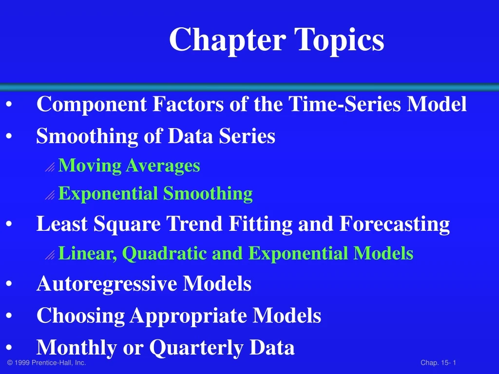
Chapter Topics • Component Factors of the Time-Series Model • Smoothing of Data Series • Moving Averages • Exponential Smoothing • Least Square Trend Fitting and Forecasting • Linear, Quadratic and Exponential Models • Autoregressive Models • Choosing Appropriate Models • Monthly or Quarterly Data
What Is Time-Series • A Quantitative Forecasting Method to Predict Future Values • Numerical Data Obtained at Regular Time Intervals • Projections Based on Past and Present Observations • Example: Year: 1994 1995 1996 1997 1998 Sales: 75.3 74.2 78.5 79.7 80.2
Time-Series Components Trend Cyclical Time-Series Seasonal Random
Trend Component • Overall Upward or Downward Movement • Data Taken Over a Period of Years Upward trend Sales Time
Cyclical Component • Upward or Downward Swings • May Vary in Length • Usually Lasts 2 - 10 Years Sales Cycle Time
Seasonal Component • Upward or Downward Swings • Regular Patterns • Observed Within 1 Year Winter Sales Time (Monthly or Quarterly)
Random or Irregular Component • Erratic, Nonsystematic, Random, ‘Residual’ Fluctuations • Due to Random Variations of • Nature • Accidents • Short Duration and Non-repeating
Multiplicative Time-Series Model • Used Primarily for Forecasting • Observed Value in Time Series is the product of Components • For Annual Data: • For Quarterly or Monthly Data: Ti= Trend Ci= Cyclical Ii= Irregular Si= Seasonal
Moving Averages • Used for Smoothing • Series of Arithmetic Means Over Time • Result Dependent Upon Choice of L, Length of Period for Computing Means • For Annual Time-Series, L Should be Odd • Example: 3-year Moving Average • First Average: • Second Average:
Moving Average Example John is a building contractor with a record of a total of 24 single family homes constructed over a 6 year period. Provide John with a Moving Average Graph. Year Units Moving Ave 1994 2 NA 1995 53 1996 23 1997 23.67 1998 7 5 1999 6 NA
Moving Average Example Solution Year Response Moving Ave 1994 2 NA 1995 53 1996 23 1997 23.67 1998 7 5 1999 6 NA Sales 8 6 4 2 0 94 95 96 97 98 99
Exponential Smoothing • Weighted Moving Average • Weights Decline Exponentially • Most Recent Observation Weighted Most • Used for Smoothing and Short Term Forecasting • Weights Are: • Subjectively Chosen • Ranges from 0 to 1 • Close to 0 for Smoothing • Close to 1 for Forecasting
Exponential Weight: Example Year Response Smoothing ValueForecast(W = .2)1994 2 2NA 1995 5(.2)(5) + (.8)(2) = 2.6 2 1996 2(.2)(2) + (.8)(2.6) = 2.48 2.6 1997 2(.2)(2) + (.8)(2.48) = 2.384 2.48 1998 7 (.2)(7) + (.8)(2.384) = 3.307 2.384 1999 6 (.2)(6) + (.8)(3.307) = 3.8463.307
Exponential Weight: Example Graph Sales 8 6 4 2 0 Data Smoothed 94 95 96 97 98 99 Year
The Linear Trend Model Year Coded Sales 94 0 2 95 1 5 96 2 2 97 3 2 98 4 7 99 5 6 Projected to year 2000 Excel Output
The Quadratic Trend Model Year Coded Sales 94 0 2 95 1 5 96 2 2 97 3 2 98 4 7 99 5 6 Excel Output
Autogregressive Modeling • Used for Forecasting • Takes Advantage of Autocorrelation • 1st order - correlation between consecutive values • 2nd order - correlation between values 2 periods apart • Autoregressive Model for pth order: Random Error
Autoregressive Model: Example The Office Concept Corp. has acquired a number of office units (in thousands of square feet) over the last 8 years. Develop the 2nd order Autoregressive models. Year Units 92 4 93 3 94 2 95 3 96 2 97 2 98 4 99 6
Autoregressive Model: Example Solution • Develop the 2nd order table • Use Excel to run a regression model Year YiYi-1Yi-2 92 4 --- --- 93 3 4 --- 94 2 3 4 95 3 2 3 96 2 32 97 2 2 3 98 4 2 2 99 6 4 2 Excel Output
Autoregressive Model Example: Forecasting Use the 2nd order model to forecast number of units for 2000:
Autoregressive Modeling Steps • 1. Choose p: Note that df = n - 2p - 1 • 2. Form a series of “lag predictor” variables • Yi-1 , Yi-2, … Yi-p • 3. Use Excel to run regression model using all p variables • 4. Test significance of Ap • If null hypothesis rejected, this model is selected • If null hypothesis not rejected, decrease p by 1 and repeat
Selecting A Forecasting Model • Perform A Residual Analysis • Look for pattern or direction • Measure Sum Square Errors - SSE (residual errors) • Measure Residual Errors Using MAD • Use Simplest Model • Principle of Parsimony
Residual Analysis e e 0 0 T T Random errors Cyclical effects not accounted for e e 0 0 T T Trend not accounted for Seasonal effects not accounted for
Measuring Errors • Sum Square Error (SSE) • Mean Absolute Deviation (MAD)