Download

1 / 28
290 likes | 371 Views
Normalised Least Mean-Square Adaptive Filtering. LMS Filtering. The update equation for the LMS algorithm is which is derived from SD as an approximation where the step size is originally considered for a deterministic gradient.

E N D
Normalised Least Mean-SquareAdaptive Filtering ELE 774 - Adaptive Signal Processing
LMS Filtering • The update equation for the LMS algorithm is which is derived from SD as an approximation where the step size is originally considered for a deterministic gradient. • LMS suffers from gradient noise due to its random nature. • Above update is problematic due to this noise • Gradient noise amplification when ||u(n)|| is large. Step size Error signal Filter input Step size ELE 774 - Adaptive Signal Processing
Normalised LMS • u(n) is random → instantaneous samples can assume any value for the norm ||u(n)|| which can be very large. • Solution: input samples can be forced to have constant norm • Normalisation • Update equation for the normalised LMS algorithm. • Note the similarity bw. NLMS and LMS update eqn.s • NLMS can be considered same as LMS except time-varying step size. ELE 774 - Adaptive Signal Processing
Normalised LMS • Block diagram very similar to that of LMS • The difference is in the Weight-Control Mechanism block. ELE 774 - Adaptive Signal Processing
Normalised LMS • We have seen that LMS algorithm optimises the H∞ criterion instead of MSE. • Similarly, NLMS optimises another problem: • From one iteration to the next, the weight vector of an adaptive filter should be changed in a minimal manner, subject to a constraint imposed on the updated filter’s output. • Mathematically, • which can be optimised by the method Lagrange multipliers ELE 774 - Adaptive Signal Processing
Normalised LMS • 1. Take the first derivative of J(n) wrt and set to zero to find • 2. Substitute this result into the constraint to solve for the multiplier • 3. Combining these results and adding a step-size parameter to control the progress gives • 4. Hence the update eqn. for NLMS becomes ELE 774 - Adaptive Signal Processing
Normalised LMS • Observations: • We may view an NLMS filter as an LMS filter with a time-varying step-size parameter • Rate of convergence of NLMS is faster than LMS • ||u(n)|| can be very large, however, likewise it can also be very small • Causes problem since it appears in the denominator • Solution: include a small correction term to avoid stability problems. ELE 774 - Adaptive Signal Processing
Normalised LMS ELE 774 - Adaptive Signal Processing
Stability of NLMS • What should be the value of step size for convergence? • Assume that the desired response is governed by • Substituting the weight-error vector into the NLMS update equation we get which provides the update for the mean-square deviation • Undisturbed error signal ELE 774 - Adaptive Signal Processing
Stability of NLMS • Find the range for so that • Right hand side is a quadratic function of , • is satisfied when • Differentiate wrt and equate to 0 to find opt • This step size yields maximum drop in the MSD! • For clarity of notation assume real-valued signals ELE 774 - Adaptive Signal Processing
Stability of NLMS • Assumption I: The fluctuations in the input signal energy ||u(n)||2 from one iteration to the next are small enough so that Then • Assumption II: Undisturbed error signal u(n) is uncorrelated with the disturbance noise (n) Then e(n): observable, u(n): unobservable ELE 774 - Adaptive Signal Processing
Stability of NLMS • Assumption III: The spectral content of the input signal u(n) is essentially flat over a frequency band larger than that occupied by each element of the weight-error vector (n) , hence • Then ELE 774 - Adaptive Signal Processing
Block LMS • In conventional LMS, filter coefficients are updated for each sample • What happens if we update the filter in every L samples? ELE 774 - Adaptive Signal Processing
Block LMS • Express the sample time n in terms of the block index k • Stack the L consecutive samples of the input signal vector u(n) into a matrix corresponding to the k-th block • where the whole k-th block will be processed by the filter i=0 i=1 i=L-1 convolution ELE 774 - Adaptive Signal Processing
Block LMS • The output of the filter is • And the error signal is • Error is generated for every sample in a block! Filter length: M=6 Block size: L=4 ELE 774 - Adaptive Signal Processing
Block LMS • Example: • M=L=3 • (k-1), k, (k+1)th block ELE 774 - Adaptive Signal Processing
Block LMS Algorithm • Conventional LMS algorithm is • For a block of length L, w(k) is fixed, however, for every sample in a block we obtain separate error signals e(n). • How can we link these two? • Sum the product , i.e. • where ELE 774 - Adaptive Signal Processing
Block LMS Algorithm • Then the estimate of the gradient becomes And the block LMS update eqn. İs where Block LMS step-size Block size LMS step-size ELE 774 - Adaptive Signal Processing
Convergence of Block LMS Conventional LMS Block LMS • Main difference is the sample averaging in Block LMS • yields better estimate of the gradient vector. • Convergence rate is similiar to conventional LMS, not faster • Block LMS requires more samples for the ‘better’ gradient estimate • Same analysis done for conventional LMS can also be applied here. • Small-step size analysis ELE 774 - Adaptive Signal Processing
Convergence of Block LMS • Average time constant if B<1/max • Misadjustment same as LMS same as LMS ELE 774 - Adaptive Signal Processing
Choice of Block Size? • Block LMS introduces processing delay • Results are obtained at every L samples, L can be >>1 • What should be length of a block? • L=M: optimal choice from the viewpoint of computational complexity. • L<M: reduces processing delay, although not optimal, better computational efficiency wrt conventional LMS • L>M: redundant operations in the adaptation, estimation of the gradient uses more information than the filter itself. ELE 774 - Adaptive Signal Processing
Fast-Block LMS • Correlation is equivalent to convolution when one of the sequences is order reversed. • Linear convolution can be effectively computed using FFT • Overlap-Add, Overlap-Save methods • A natural extension of Block LMS is to use FFT • Let block size be equal to the filter length, L=M, • Use Overlap-Save method with an FFT size of N=2M. ELE 774 - Adaptive Signal Processing
Fast-Block LMS • Using these two in the convolution, for the k-th block • The Mx1 desired response vector is • and the Mx1 error vector is ELE 774 - Adaptive Signal Processing
Fast-Block LMS • Correlation is convolution with one of the seq.s order reversed: • Then the update equation becomes (in the frequency domain) • Computational Complexity: • Conventional LMS: requires 2M multiplications per sample • 2M2 multiplications per block (of length M) • Fast-Block LMS: 1 FFT = N log2(N) real multiplications (N=2M) • 5 (I)FFTs, UH(k)E(k): 4N multiplications → Total: 10Mlog2M+28M mult.s • For M=1024, Fast Block LMS is 16 times faster than conventional LMS ELE 774 - Adaptive Signal Processing
Fast-Block LMS • Same step size for all frequency bins (of FFT). • Rate of convergence can be improved by assigning separate step-size parameters to every bin • : constant, Pi: estimate of the average power in the i-th freq. Bin • Assumes wss. environment. • If not wss., use the recursion i-th input of the Fast-LMS algorithm (freq. dom.) for the k-th block ELE 774 - Adaptive Signal Processing
Fast-Block LMS • Run the iterations for all blocks to obtain • Then the step size parameter can be replace by the matrix where • Update the Fast-LMS algorithm as follows: • 1. • 2. replace by in the update eqn. ELE 774 - Adaptive Signal Processing
’ ’ ELE 774 - Adaptive Signal Processing