Download
1 / 27
360 likes | 726 Views
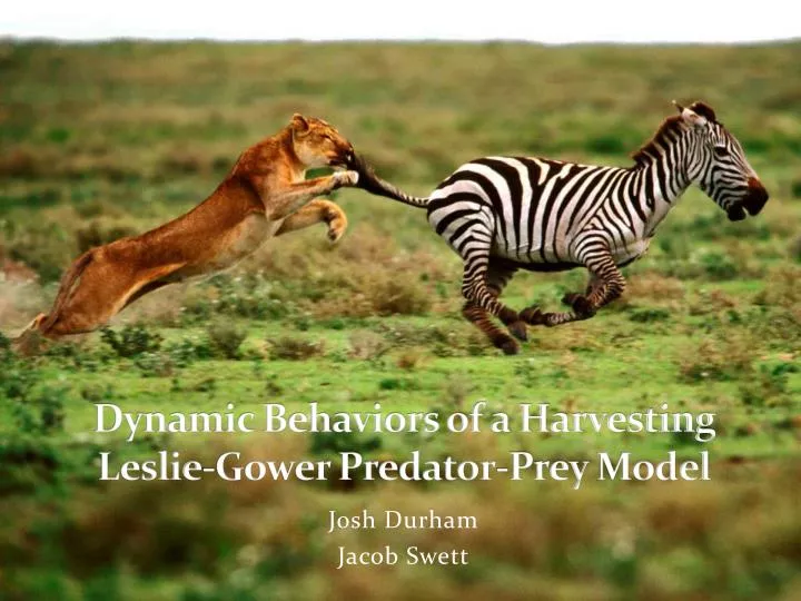
Dynamic Behaviors of a Harvesting Leslie-Gower Predator-Prey Model. Josh Durham Jacob Swett. The Article. Dynamic Behaviors of a Harvesting Leslie-Gower Predator-Prey Model Na Zhang, 1 Fengde Chen, 1 Qianqian Su, 1 and Ting Wu 2

E N D
Dynamic Behaviors of a Harvesting Leslie-Gower Predator-Prey Model Josh Durham Jacob Swett
The Article • Dynamic Behaviors of a Harvesting Leslie-Gower Predator-Prey Model • Na Zhang,1 Fengde Chen,1 Qianqian Su,1 and Ting Wu2 • 1 College of Mathematics and Computer Science, Fuzhou University, Fuzhou 350002, Fujian, China • 2 Department of Mathematics and Physics, Minjiang College, Fuzhou 350108, Fujian, China • Published in Discrete Dynamics in Nature and Society • Received 24 October 2010; Accepted 8 February 2011 • Academic Editor: Prasanta K. Panigrahi
Outline • Introduction • Stability Property of Positive Equilibrium • The Influence of Harvesting • Bionomic Equilibrium • Optimal Harvesting Policy • Numerical Example • Conclusions • Questions
Predatory Prey Model • – density of prey species • – density or predator species • - intrinsic growth rate for prey and predator, respectively • - catch rate • - competition rate • - prey conversion rate • is the carrying capacity of the prey • is the prey-dependent carrying capacity of the predator
Model with Harvesting • - constant effort spent by harvesting agency on the prey • - constant effort spent by harvesting agency on the predator • Assume:
Why Study a Harvesting Model? • The harvesting of biological resources commonly occurs in: • Fisheries • Forestry • Wildlife management • Allows for predictions given various assumptions • Important for optimization
Stability Property of Positive Equilibrium • Given that the harvesting remains strictly less than the intrinsic growth rate, the system under study has a unique positive equilibrium • Satisfies the following equalities • ,
What does this mean? • It means that the positive equilibrium of the system under study is locally asymptotically stable • Stability is the same as what we have discussed in class • The proof of this is very similar to examples that we have done in class. • First, find the Jacobian
Proof Continued • Then we find the characteristic equation • Given the above information, we can see that the unique positive equilibrium of the system is stable
Global Stability • The positive equilibrium is globally stable • The proof of this fact is beyond the scope of this course • Instead, there will be a brief summary of major points • Equilibrium dependent only on coefficients of system • Lyapunov Function • Lyapunov’s asymptotic stability theorem
Influence of Harvesting • Case 1: Harvesting only prey species • Case 2: Harvesting only predator species
Case 3: Harvesting predator and prey together • Difficult to give a detailed analysis of all possible cases so the focus will be on answering • Whether or not it is possible to choose harvesting parameters such that the harvesting of predator and prey will not cause a change in density of the prey species over time • If it is possible, what will the dynamic behaviors of the predator species be? • We find that: allows the first question to be answered with, yes • We also find that by substituting the above equality into the predator equation, it will lead to a decrease in the predator species
Bionomic Equilibrium • Biological equilibrium + Economic equilibrium=Bionomic equilibrium • Biological equilibrium: • Economic equilibrium: • TR = TC • TR is the total revenue obtained by selling the harvested predators and prey • TC is the total cost for the effort of harvesting both predators and prey
Bionomic Equilibrium (Cont.) • We will define four new variables: • p1 is the price per unit biomass of the prey H • p2 is the price per unit biomass of the predator P • q1 is the fishing cost per unit effort of the prey H • q2 is the fishing cost per unit effort of the predator P • The revenue from harvesting can written as: • Where: and • And: and
Bionomic Equilibrium (Cont.) • The revenue from harvesting equation and the predator and prey equations must all be considered together: • Price per unit biomass (p1,2) and the fishing cost per unit effort (q1,2) are assumed to be constant • Since the total revenue (TR) and total cost (TC) are not determined, four cases will be considered to determine bionomic equilibrium
Case I • That is: • In other words the revenue () is less than the cost () for harvesting prey and it will be stopped (i.e. c1 = 0) • Thus, • Predator harvesting will continue as long as • To determine equilibrium: • Solve for P • Substitute it into the predator equation • Substitute the predator equation and P into the prey equation • Simplify • Thus, if r1 > a2(q2/p2) and r2 > (a2b1q2/r1q2) both hold, then bionomic equilibrium is obtained.
Case II • That is: • In other words the revenue () is less than the cost () for harvesting predators and it will be stopped (i.e. c2= 0) • Thus, • Prey harvesting will continue as long as • Example: • Sub H into predator equation , • Yields: • Substituting H and P into the prey equation, • Yields: • Thus, if r1 > ((a1r2 – a2b1)q1/a2p1) holds then bionomic equilibrium is obtained for this case.
Case III • and • That is to say, the total costs exceeds the revenue for both predators and prey • No profit • Clearly c1 = c2 = 0 • No bionomic equilibrium
Case IV • and • That is: and • Solve as before • Thus if and hold then bionomic equilibrium is obtained. • It becomes obvious that bionomic equilibrium may occur if the intrinsic growth rates of the predators and prey exceed the values calculated
Optimal Harvesting Policy • To determine an optimal harvesting policy, a continuous time-stream of revenue function, J, is maximized: • -δ is the instantaneous annual rate of discount • c1(t) and c2(t) are the control variables • The assumption: ; still holds • Pontryagin's Maximum Principle is invoked to maximize the equation
Pontryagin's Maximum Principle • A method for the computation of optimal controls • The Maximum Principle can be thought of as a far reaching generalization of the classical subject of the calculus of variations
Results and Implications • Applying Pontryagin's Maximum Principle to the revenue function J, shows that optimal equilibrium effort levels (c1 and c2)are obtained when: • Recall: • - intrinsic growth rate for prey and predator, respectively • - catch rate • - competition rate • - prey conversion rate
Numerical Example • Using the following values as inputs into the optimized equation: • Gives: • Solving with Maple, the authors obtained:
Numerical Example (Cont.) • From the previous results only one results meets the following conditions: • Namely: • These values can then be entered into the predator-prey harvesting equation
Numerical Example (Cont.) • Substituting the values for H and P into the below equations: • And rearranging to solve for c1 and c2, gives:
Conclusions • Introduced a harvesting Leslie-Gower predator-prey model • The system discussed was globally stable • Provided an analysis of some effects of different harvesting policies • Considered economic profit of harvesting • Results show that optimal harvesting policies may exist • Demonstrate that the optimal harvesting policy is attainable