Sensor Network Simulation ( Sensim) Components Analysis

1. Sensor Network Simulation( Sensim) Components Analysis • AICIP Research Group Presentation Yang Liu

2. Design Goal • Parallel discrete event sensor network simulator • Scale to thousands of sensor nodes • Provide energy consumption computation • Integrate typical protocols of sensor networks ( MAC, network, application ), adopt an open architecture for future protocol implementation • Easy to operate, easy to understand • ACA design, large dataset visualization

3. What to Simulate? • Metrics for sensor network • Three prospective • Individual • Group ( regional) • Network wide • Metrics • Throughput • Power consumption • Time ( Latency, lifetime, idle time, transmitting and receiving time etc.) • QOS ( packet loss, Coverage, and sensor network failure)

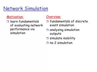
4. How to Simulate? • A brief simulation architecture

5. Parallelization • Using Message Passing Interface (MPI) Standard and PC cluster to realize parallel simulation. • We choose MPICH-1.2.5.2 library. • PC cluster: peacock, P1, P2, and P3. • * How to decompose work ?

6. Parallel Algorithm Design • Typical techniques • Data parallel model: • Identical operations applied concurrently on different data • Task-Graph Model • Different processes are executing different tasks ( static mapping) • Work-Pool Model • Dynamic mapping tasks to processes • Work-Manage Model • One process generates and distributes work to others • Producer-Consumer Model • Data is passed through several processes, each perform a different task just like pipeline

7. Our Case • Scale to thousands of sensor nodes, memory is a big issue. • The tasks are high correlated, therefore it is hard to partition. • Data parallel model is desirable. • In our case, to partition sensor nodes based on region

8. Work Decomposition • Region based partition ( histogram) • Maximize data locality • Minimize volume of data exchange • Minimize frequency of interactions XY 2D Partition Y axis Partition X axis Partition

9. Overlapping Communication and computation • Initiate communication ( MPI_Isend/MPI_Irecv) • Calculate inner values • Finish communication ( MPI_Waitall) • Calculate boundary values One ghost cell N-ghost zone

10. Battery Model • Linear Model: • U: current capacity U’: previous capacity i(t): instantaneous current • Non-Linear Model: [2] • T: discharged time; K, h: constants depending on cell design and chemical architecture of battery; Va: average value of the cell voltage during the discharge; I: discharge current;

11. Battery Model (cont.) • Pulsed Discharge Model [1] • Relaxation phenomena • If battery is allowed to relax, lost capacity can be recovered. • Binary Pulsed Discharge Model • - Based on Binary Markov Chain • Generalized Pulsed Discharge Model

12. Energy Consumption Model • Some experiment data [3][4]

13. Energy Consumption Model (cont.) • Simple energy model • Energy spent in transmission = (edda + et)b • Energy spent in reception =erb • Energy spent sensing =esb • Energy spent in computation ( leakage current model)[6] • Depends on the total capacitance switched and the number of cycles the program • takes • ed is the energy dissipated per bit per m2 (amplifier) • et is the energy spent by transmission circuitry per bit • eris the energy spent by reception circuitry per bit • es is the energy spent sensing per bit • b is number of bits to transmit or receive • t is the time • α is a constant 2(will use the common values of α=2 and α=4) • d is the transmitting distance

14. PHY Layer Abstraction • Radio Propagation Model: [5] • Outdoor propagation Model: • Free Space Model: • Pf : transmitted signal power • Pr : receive signal power • Gt Gr : antenna gains of transmitter and receiver respectively • L is system loss ( L > 1) • λ : wavelength • d : distance from transmitter

15. PHY Layer Abstraction (cont.) • Ground Reflection (Two-Ray) • Faster power loss as distance increase • ht hr are the height of the transmit and receive antennas respectively • Cross-over distance dc • d < dc free space use else two-ray model

16. PHY Layer Abstraction (cont.) • Indoor Propagation Model: • Shadowing model. • Underwater Acoustic Propagation Model:

17. Mac Layer Abstraction • Typical protocols • Contention-based protocols • IEEE 802.11 • PAMAS • S-MAC • TDMA

18. MAC Layer Abstraction (cont.) • Take S – Mac as an example • Energy consumption abstraction • Three states: receive, transmit, sleep • Broadcast: • Point-to-point: RTS/CTS/ACK • Sender • receiver

19. Mac Layer Abstraction (cont.) • Latency computation • Carrier sense delay • Backoff delay • Transmission delay • Propagation delay • Sleep delay • Queuing delay • Processing delay

20. Queuing Model • Discrete time queuing models • Models • Depending on arrival and departure processes • Geo/Geo/1/ and Geo/Geo/1/N • M/M/1

21. Queuing Model (cont.) • Geo/Geo/1 and Geo/Geo/1/N queue model • Geo/Geo/1 Geo/Geo/1/N • M/M/1 queue model • M/M/1 Geo/Geo/1

22. Network Layer Abstraction • Protocols: • Flooding -SPIN • Gradient – Directed Diffusion • Clustering - LEACH • Geographic -GEAR • Energy aware - SPIN-EC, LEACH, GEAR • Highlight • Route setting up overhead • Communication Pattern (unicast, multicast, broadcast) • Packet transmitted

23. Middleware Abstraction • Agent-based architecture • Client/Server based architecture • In-network processing scheme • Query system

24. APP Layer Abstraction • Traffic Generation Model • CBT • Constant bit rate transfer : Home surveillance, parking • lot sensor network application • Target detection and tracking • Moving target Models: • 1. Given start point, moving in straight line at constant speed. When arriving the edge, change the direction by “bouncing” off the virtual wall. • 2. Moving target is given an initial location along with a series of waypoints

25. Topology Generation Model • GT-ITM, Tiers Model • Concern with the hierarchical properties of • Internet • Inet, PLRG • Connectivity properties • BRITE • Hierarchical properties, degree distributions, • Connectivity properties

26. Large Data Set Visualization • Large memory and high speed requirement for sensor networks visualization • Hierarchy sensor data rendering • Higher level – region based information • Energy consumption map, Traffic distribution map • simulation data report based on the whole area etc. • Lower Level – portion of sensor nodes information • Detailed information of sensor nodes • Graph tools

27. References • [1] C.F.Chiasserini and R.R.Rao, “Pulsed Battery Discharge in Communication Devices”, MobiCOM , 1999. • [2] H.D.Linden, “Handbook of Batteries”, 2nd ED. McGrawHill, 1995 • [3] Vijay Raghunathan, Curt Schurgers, Sung Park, Mani B. Srivastava.  “Energy –aware wireless micro sensor networks." IEEE Signal Processing Magazine, Volume: 19 Issue: 2, Mar 2002. • [4] A. Mainwaring, D. Culler, J. Polastre, R. Szewczyk, J. Anderson. "Wireless Sensor Networks for Habitat Monitoring," Proceedings of the First ACM International Workshop on Wireless Sensor Networks and Applications (WSNA '02), Georgia, September 2002. • [5] T.S.Rappaport, “Wireless communications principles and practice”, Prentice Hall 2002 • [6] A.sinha and A. Chandrakasan, “Energy Aware Software”, Proceedings of the 13th International Conference on VLSI Design, 2000