But it's pure0 so this branch ends

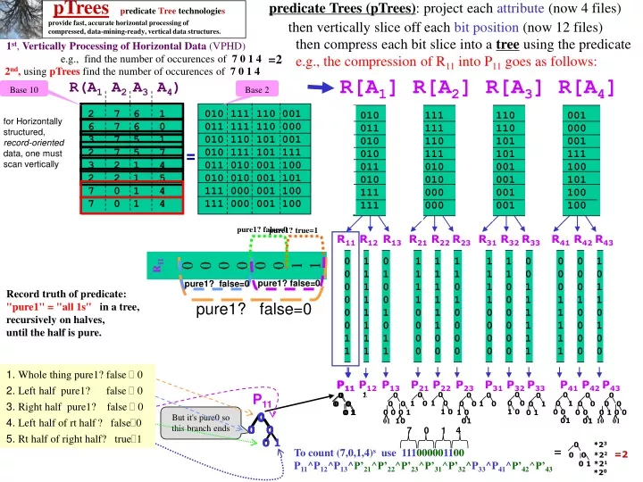
1. pTreespredicateTreetechnologies provide fast, accurate horizontal processing of compressed, data-mining-ready, vertical data structures. predicate Trees (pTrees): project each attribute (now 4 files) 1st, Vertically Processing of Horizontal Data (VPHD) R[A1] R[A2] R[A3] R[A4] R(A1 A2 A3 A4) 2 7 6 1 6 7 6 0 3 7 5 1 2 7 5 7 3 2 1 4 2 2 1 5 7 0 1 4 7 0 1 4 010 111 110 001 011 111 110 000 010 110 101 001 010 111 101 111 011 010 001 100 010 010 001 101 111 000 001 100 111 000 001 100 010 111 110 001 011 111 110 000 010 110 101 001 010 111 101 111 011 010 001 100 010 010 001 101 111 000 001 100 111 000 001 100 for Horizontally structured, record-oriented data, one must scan vertically = pure1? true=1 pure1? false=0 R11 R12 R13 R21 R22 R23 R31 R32 R33 R41 R42 R43 0 1 0 1 1 1 1 1 0 0 0 1 0 1 1 1 1 1 1 1 0 0 0 0 0 1 0 1 1 0 1 0 1 0 0 1 0 1 0 1 1 1 1 0 1 1 1 1 0 1 1 0 1 0 0 0 1 1 0 0 0 1 0 0 1 0 0 0 1 1 0 1 1 1 1 0 0 0 0 0 1 1 0 0 1 1 1 0 0 0 0 0 1 1 0 0 pure1? false=0 pure1? false=0 pure1? false=0 0 0 0 1 0 01 0 1 0 1 0 1 1. Whole thing pure1? false  0 P11 P12 P13 P21 P22 P23 P31 P32 P33 P41 P42 P43 2. Left half pure1? false  0 P11 0 0 0 0 0 01 3. Right half pure1? false  0 0 0 0 0 1 0 0 10 01 0 0 0 1 0 0 0 0 0 0 0 1 01 10 0 0 0 0 1 0 0 0 0 1 0 0 0 0 1 0 0 0 0 0 0 0 0 0 0 1 0 0 ^ ^ ^ ^ ^ ^ ^ 0 0 1 0 1 4. Left half of rt half? false0 7 0 1 4 0 0 1 0 0 01 5. Rt half of right half? true1 0 *23 0 0 *22 =2 0 1 *21 *20 0 1 0 To count (7,0,1,4)s use 111000001100P11^P12^P13^P’21^P’22^P’23^P’31^P’32^P33^P41^P’42^P’43 = then vertically slice off each bit position (now 12 files) then compress each bit slice into a treeusing the predicate e.g., the compression of R11 into P11 goes as follows: =2 e.g., find the number of occurences of 7 0 1 4 2nd, using pTreesfind the number of occurences of 7 0 1 4 Base 10 Base 2 R11 0 0 0 0 0 0 1 1 Record truth of predicate: "pure1" = "all 1s" in a tree, recursively on halves, until the half is pure. P11 But it's pure0 so this branch ends

2. R(A1 A2 A3 A4) R11 R12 R13 R21 R22 R23 R31 R32 R33 R41 R42 R43 To count occurrences of 7,0,1,4 use 111000001100: 0 P11^P12^P13^P’21^P’22^P’23^P’31^P’32^P33^P41^P’42^P’43 = 0 0 01 0 0 ^ 0 0 0 1 0 0 0 0 Top-down construction of basic pTrees is best for understanding, bottom-up is much faster (once across). 1 0 0 1 0 1 0 0 0 0 1 0 01 1 1 0 1 0 0 1 01 R11 R12 R13 R21 R22 R23 R31 R32 R33 R41 R42 R43 This (terminal) 0 makes entire left branch 0 There is no need to look at the other operands. 0 1 0 1 1 1 1 1 0 0 0 1 0 1 1 1 1 1 1 1 0 0 0 0 0 1 0 1 1 0 1 0 1 0 0 1 0 1 0 1 1 1 1 0 1 1 1 1 1 0 1 0 1 0 0 0 1 1 0 0 0 1 0 0 1 0 0 0 1 1 0 1 1 1 1 0 0 0 0 0 1 1 0 0 1 1 1 0 0 0 0 0 1 1 0 0 7 0 1 4 These 0s make this node 0 P11 P12 P13 P21 P22 P23 P31 P32 P33 P41 P42 P43 These 1s and these 0s(which when complemented are 1's)make node1 0 0 0 0 0 01 0 0 0 0 1 0 0 10 01 0 0 0 1 0 0 0 0 0 0 0 1 01 10 0 0 0 0 1 10 0 1 0 ^ ^ ^ ^ ^ ^ ^ ^ ^ 0 0 1 0 1 0 0 1 0 0 01 0 1 0 0 1 0 1 1 1 1 1 0 0 0 1 0 1 1 1 1 1 1 1 0 0 0 0 0 1 0 1 1 0 1 0 1 0 0 1 0 1 0 1 1 1 1 0 1 1 1 1 1 0 1 0 1 0 0 0 1 1 0 0 0 1 0 0 1 0 0 0 1 1 0 1 1 1 1 0 0 0 0 0 1 1 0 0 1 1 1 0 0 0 0 0 1 1 0 0 010 111 110 001 011 111 110 000 010 110 101 001 010 111 101 111 101 010 001 100 010 010 001 101 111 000 001 100 111 000 001 100 2 7 6 1 3 7 6 0 2 7 5 1 2 7 5 7 5 2 1 4 2 2 1 5 7 0 1 4 7 0 1 4 = # change The 21-level has the only 1-bit so 1-count=1*21 =2 R11 0 0 0 0 1 0 1 1 Bottom-up construction of 1-Dim, P11, is done using in-order tree traversal, collapsing of pure siblings as we go: P11 0 Siblings are pure0 so collapse!

3. stride=8 stride=4 stride=2 stride=1 (raw) P11 P11 P11 P23 P21 P41 P12 P31 P13 P43 P42 P12 P22 P23 P12 P42 P21 P31 P43 P41 P22 P23 P13 P22 P21 P13 P43 P42 P41 P31 ^ ^ ^ ^ ^ ^ ^ ^ ^ ^ ^ ^ ^ ^ ^ ^ ^ ^ ^ ^ ^ ^ ^ ^ ^ ^ ^ Store complements or derive them when needed? Or process complement set with separate code? P11^P12^P13^P’21^P’22^P’23^P’31^P’32^P33^P41^P’42^P’43 Pure1 stride= 4  7,0,1,4=111000001100 Pure0 stride= 4  Mixed stride= 4  P32 P32 P33 P33 P33 P32 P11 P41 P21 P22 P23 P31 P32 P42 P43 P12 P13 P33 0 1 0 1 0 0 0 0 1 0 01 0 0 0 0 0 01 0 0 0 1 0 01 0 1 0 1 0 0 0 0 1 0 01 0 1 0 1 0 0 0 0 0 0 01 0 0 1 0 0 01 0 0 1 0 0 01 0 0 0 0 0 01 0 0 1 0 0 01 0 0 0 1 1 0 1 0 0 0 1 0 0 0 0 0 0 0 1 0 1 0 0 1 0 1 0 0 1 01 0 1 0 0 1 01 0 1 0 0 1 01 1 0 0 0 0 1 0 0 0 1 0 1 0 1 0 1 0 0 0 0 0 0 0 0 Retrieve stride=2 vectors: st=2_P112 st=2_P122 st=2_P132 st=2_P’222 st=2_P’432 0 1 1 0 0 0 0 1 1 0 0 0 1 0 1 0 1 1 0 1 0 1 1 0 PureOne stride= 2  Derive comps: Mix of comp-no change. Swap p1, p0 0 1 0 1 0 1 0 1 0 1 P11 P41 P’21 P’22 P’23 P’31 P’32 P’42 P’43 P12 P13 P33 7 0 1 4 0 0 PureZero stride= 2  0 0 0 0 1 0 0 1 Pure1 stride= 4  0 0 0 1 0 1 0 0 0 1 0 1 0 1 0 1 0 0 1 0 1 0 0 1 0 0 0 1 0 0 0 1 0 1 0 0 1 0 1 0 0 0 1 0 0 0 1 0 1 0 0 0 1 0 Pure0 stride= 4  1 0 0 0 0 0 0 0 0 0 1 0 0 10 01 0 0 0 0 0 0 1 01 10 0 0 0 0 1 0 0 10 01 0 0 0 0 0 0 1 01 10 0 0 0 0 0 0 1 01 10 0 0 0 0 1 0 0 10 01 0 0 0 0 1 10 0 0 0 0 1 10 0 0 0 0 1 10 0 0 0 0 1 0 1 0 0 0 1 0 0 0 0 0 0 0 Mixed stride= 4  0 1 1 0 0 0 0 1 1 0 0 0 1 0 1 0 1 1 0 1 0 1 1 0 0 1 0 0 1 0 0 1 0 0 1 0 0 1 0 0 1 0 A Mixed pTree is the AND of the complements of the pure1 and pure0. Derive and store? Any 1 of Pure1, Pure0, Mixed is derivable from others. Store 2? Store all? If there is a stride, it is level-1. Retrieve stride=2 (or stride=1's) only if stride=4 has 0-bit. Count contribution computable from these: 2*Count( & Pure1_str=4)=4*Count(0 0)=4*0= 0 And then for each individual pTree, retrieve that stride=2 vector only if Pure1 stride=4 has a 0-bit there. So retrieve: P112 P122 P132 P’222 P’432 The contribution to the result 1-bit count from level 1: 21 * Count( & Pure1_lev1 ) = 2 * Count( 0 1 ) = 2* 1 = 2 Retrieve level 0 vector only if orPure0_lev1 (=11) has a 0-bit in that position. And then for each individual pTree, retrieve that level_0 vector only if Pure1_lev1 has a 0-bit there. Since orPure0_lev1 )=(11) has no zero-bits, no level_0 vectors need to be retrieved. The answer, then, is 0 + 2 = 2. Binary pTrees are used here for better understanding. In reality, the "stride" of each level would be tuned to processor architecture. E.g., on 64-bit processors, it would make sense to have only 2 levels, where each level_1 bit "covers" or "is the predicate truth of" a string of 64 consecutive raw bits. An alternative is to tune coverages to cache strides. In any case, we suggest storing level_0 (raw) in its entirety and building level_1 pTrees using various predicates (e.g., pure1, pure0, mixed, gt50, gt10). Then only if the tables are very very deep, build level_2s on top of that... Last point: Level_1s can be used independently of level_0s to do "approximate but very fast" data mining (especially using the gt50 predicate).

4. R11 0 0 0 0 1 0 1 1 pTrees construction [one-time] 0 0 0 0 1 1 1 1 1 0 0 0 1 0 0 1 0 1 0 0 0 1 0 0 0 0 0 0 0 0 (changed R11 so this issue of recording 1-counts as you go is pertinent) • 1-child is pure1 and 0-child is just below 50% (so parent_node=1) • 1-child is just above 50% and the 0-child has almost no 1-bits (so that the parent node=0). (example on next slide). R11 R12 R13 R21 R22 R23 R31 R32 R33 R41 R42 R43 1 0 0 0 1 1 1 1 1 1 1 1 1 1 0 1 1 1 1 1 0 0 0 1 0 1 1 1 1 1 1 1 0 0 0 0 0 1 0 1 1 0 1 0 1 0 0 1 0 1 0 1 1 1 1 0 1 1 1 1 1 0 1 0 1 0 0 0 1 1 0 0 0 1 0 0 1 0 0 0 1 1 0 1 1 1 1 0 0 0 0 0 1 1 0 0 1 1 1 0 0 0 0 0 1 1 0 0 Can be done as 1 pass thru each bit slice required for bottom-up construction of pure1 pTrees. R11 R12 R13 R21 R22 R23 R31 R32 R33 R41 R42 R43 gte50_pTree11 0 1 0 1 1 1 1 1 0 0 0 1 0 1 1 1 1 1 1 1 0 0 0 0 0 1 0 1 1 0 1 0 1 0 0 1 0 1 0 1 1 1 1 0 1 1 1 1 1 0 1 0 1 0 0 0 1 1 0 0 0 1 0 0 1 0 0 0 1 1 0 1 1 1 1 0 0 0 0 0 1 1 0 0 1 1 1 0 0 0 0 0 1 1 0 0 0 gte100_pTree11 0 We must record 1-count of the stride of each inode (e.g., in binary trees, if one child=1 and the other=0, it could be the 1-child is pure1 and the 0-child is just below 50% (so parent_node=1) or the 1-child is just above 50% and the 0-child has almost no 1-bits (so parent node=0). R11 1 0 0 0 1 0 1 1 8_4_2_1_gte50%_pTree11 1 0 or 1? Need to know left branch OneCount=1, and right branch Onecount=3. So this stride=8 subtree OneCount=4 ( 50%). 0 or 1? OneCount of left branch=1, of right branch=0. So stride=4 subtree OneCount=1 (< 50%). OneCount of right branch=0 (pure0), but OneCount of left branch=?. Finally, recording the OneCounts as we build the tree upwards is a near-zero-extra-cost step.

5. Multi-level pTrees A predicate map or pMap is a n-bit-string derived from a cardinality=n data table (having n rows). Any pMap requires two choices: 1. An ordering for the table rows (e.g., raster-row or raster-column, and for spatial data, Z-AKA-Peano or Hilbert). This ordering is typically the same for all pMaps derived from the same table. 2. A predicate (which evaluates to t/f on any row. A pTree (made up of a raw pMap (level-0) as defined above and a level-1 pMap) requires a third choice: 3. A stride length. A level-1 pMap is a bit-string derived by applying a predicate to consecutive strides (contiguous subsets) of a raw pMap. Typical predicates for a level-1 pMaps include: "purely-one-bits in each stride", "purely-zero-bits" and "x%-one-bits" in each stride.

6. R11 1 0 0 0 1 0 1 1 construction [revisited with the new definitions] level-1 gt50 stride=8 pMap level-1 gt50 stride=4 pMap 0 1 1 1 0 1 0 1 0 0 0 1 1 1 gt50_pTrees11 raw level-0 pMap 1

7. gte50 Satlog-Landsat stride=64, classes: redsoil cotton greysoil dampgreysoil stubble verydampgreysoil 320-bit strides start end cls cls 320 stride 2 1073 1 1 2 321 1074 1552 2 1 322 641 1553 2513 3 1 642 961 2514 2928 4 2 1074 1393 2929 3398 5 3 1553 1872 3399 4435 _7 3 1873 2192 4436 3 2193 2512 4 2514 2833 5 2929 3248 7 3399 3718 7 3719 4038 7 4039 4358 0 0 0 0 0 0 1 2 1 1 1 1 ... ... ... ... ... ... 255 255 255 255 255 255 r r r r c c c c g g g g d d d d s s s s v v v v cl cl cl cl 1 1 1 1 0 0 0 0 0 0 0 0 0 0 0 0 0 0 0 0 0 0 0 0 0 0 0 0 0 0 0 0 0 0 0 0 1 0 0 1 1 0 0 0 0 0 0 1 0 0 0 0 0 0 0 0 0 0 0 0 1 1 0 0 1 0 1 0 0 0 0 0 0 0 0 0 0 0 0 0 0 0 0 0 0 0 0 0 0 0 0 0 0 0 0 0 Rclass ir1class ir2class Gclass ir2 ir2 ir1 G ir2 ir1 0 0 0 0 0 0 0 1 0 0 0 0 0 0 0 0 0 0 0 0 0 0 0 0 0 0 1 0 0 0 0 0 0 0 1 1 1 1 1 1 1 1 1 1 0 0 0 0 0 1 0 0 0 0 0 0 0 0 0 0 0 1 1 0 0 0 0 0 R G ir1 ir2 cls means stds means stds means stds means stds 1 64.33 6.80 104.33 3.77 112.67 0.94 100.00 16.31 2 46.00 0.00 35.00 0.00 98.00 0.00 66.00 0.00 3 89.33 1.89 101.67 3.77 101.33 3.77 85.33 3.77 4 78.00 0.00 91.00 0.00 96.00 0.00 78.00 0.00 5 57.00 0.00 53.00 0.00 66.00 0.00 57.00 0.00 7 67.67 1.70 76.33 1.89 74.00 0.00 67.67 1.70 ... ... ... ... ... ... ... ... ... ... 1 1 0 1 0 0 1 0 1 0 0 0 1 0 1 1 0 0 0 1 1 0 0 0 255 255 255 255 255 255 255 255 255 255 1 0 0 0 0 1 0 0 1 0 1 1 0 0 0 0 1 0 0 0 0 0 1 0 R ir1 R R ir2 G G G ir1 R Rir2 Gir2 ir1ir2 Rir1 RG Gir1 For gte50 Satlog-Landsat stride=320, we get: Note that for stride=320, the means are way off and it therefore will probably produce very inaccurate classification.. A level-0 pVector is a bit string with 1 bit per record. A level-1 pVector is a bit string with 1 bit per record stride which gives truth of a predicate applied to record stride. A n-level pTree consists of a level-k pVector (k=0...n-1) all with the same predicate and s.t. each level-k stride is a contained within one level-k-1 stride.

8. R 1 2 3 4 5 7 cls 14 15 16 17 18 19 20 21 22 23 24 25 26 27 28 29 30 31 32 33 34 35 36 37 38 39 1 40 41 42 1 43 1 44 2 45 46 4 47 48 49 50 51 2 52 53 1 54 55 4 56 57 1 2 58 1 59 2 60 1 61 1 62 63 64 2 2 2 65 66 1 2 2 67 1 3 68 1 1 2 69 70 2 71 1 4 72 73 74 75 76 77 78 2 79 80 81 82 83 84 2 85 86 87 88 8 89 1 90 91 92 3 93 94 95 96 97 98 99 100 101 102 103 104 105 106 107 108 109 110 111 112 113 114 115 116 117 118 119 120 121 122 123 124 125 126 G 1 2 3 4 5 7 cls 14 15 16 17 18 19 20 21 22 23 24 25 26 27 28 29 30 31 32 1 33 2 34 1 35 36 1 37 38 39 1 40 41 42 43 1 44 45 46 47 48 1 49 50 51 1 52 1 53 1 54 55 5 56 57 58 59 60 61 1 62 63 64 65 66 67 1 1 68 69 70 71 72 73 3 74 75 2 7 76 77 78 79 4 80 81 82 83 1 84 85 86 87 88 89 90 91 4 92 93 94 95 96 97 2 98 2 99 2 7 100 101 102 103 3 2 104 105 106 107 1 3 108 109 110 111 4 112 113 114 115 1 116 117 118 119 120 121 122 123 124 125 126 ir1 1 2 3 4 5 7 cls 14 15 16 17 18 19 20 21 22 23 24 25 26 27 28 29 30 31 32 33 34 35 36 37 38 39 40 41 42 43 44 45 46 47 48 49 50 51 52 53 54 55 56 57 58 59 60 61 62 63 64 1 65 2 66 2 67 1 68 1 69 70 1 71 72 1 73 1 74 1 6 75 76 77 1 78 79 2 80 81 82 1 83 84 85 86 1 87 88 89 90 91 92 1 93 94 95 96 3 1 97 1 1 98 1 99 100 1 101 1 102 103 104 6 1 105 1 106 1 107 108 109 110 111 112 6 1 113 114 3 1 3 115 116 2 1 117 118 1 119 120 121 122 4 123 124 1 125 126 ir2 1 2 3 4 5 7 cls 14 1 15 16 17 18 19 20 21 22 23 24 25 26 27 28 29 30 31 32 33 34 35 36 37 38 39 40 41 42 43 44 45 46 47 48 49 50 51 52 53 54 55 56 57 2 58 1 59 2 60 1 61 1 62 63 64 1 1 2 65 1 66 2 1 2 67 2 3 68 1 1 2 69 1 70 2 71 4 72 73 74 75 1 76 77 78 2 79 80 81 1 82 1 1 83 1 1 84 1 85 86 1 87 88 1 7 89 1 90 2 1 91 1 92 1 93 94 1 95 2 96 97 98 99 100 101 102 103 104 105 106 107 108 109 110 111 112 113 114 115 116 117 118 119 120 1 121 122 123 1 124 125 126 1 classes: 1. redsoil 2. cotton 3. greysoil 4. dampgreysoil 5. stubble 7. verydampgreysoil gte50 stride=64 FT=1, CT=.95 Strong rules AC exist.C=ClassSet, A=IntervalConf. |PA&Pc| /|PA| > CT Frequency condition |PA| > FT Frequency unimportant? There is no closure to help mine confident rules. But we can see there are strong rules: G[47,64]5 G[65,81]7 G[0,46]2 G[81,94]4 G[94,255]{1,3} R[0,48]{1,2} R[49,62]{1,5} R[63,81]{1,4,7} R[82,255]3 ir1[89,255]{1,2,3,4} ir1[0,88]{5,7} ir2[53,255]{1,2,3,4,7} ir2[0,52]5 Altho no closures exits, but we can mine confident rules by scanning values (1 pass 0-255) for each band. This is not too expensive. For an unclassified sample, let rules vote (weight inversely by consequent size and directly by std % in gap, etc.). Is there any new information in 2-hop rules, e.g., RRGG GGclscls? Can cls=1,3 be separated (only classes not separated by G). We will also try using all the strong one-class or two-class rules above.

9. G 1 2 3 4 5 7 32 1 33 2 34 1 35 36 1 37 38 39 1 40 41 42 43 1 44 45 46 47 48 1 49 50 51 1 52 1 53 1 54 55 5 56 57 58 59 60 61 1 62 63 64 65 66 67 1 1 68 69 70 71 72 73 3 74 75 2 7 76 77 78 79 4 80 81 82 83 1 84 85 86 87 88 89 90 91 4 92 93 94 95 96 97 2 98 2 99 2 7 100 101 102 103 3 2 104 105 106 107 1 3 108 109 110 111 4 112 113 114 115 1 R 145678921234567893123456789412345678951234567896123456789712345678981234567899123456789a123456789b123456789c123456 G32 33 34 35 36 37 38 39 40 41 42 43 44 45 46 47 48 49 50 51 52 53 54 55 56 57 58 59 60 61 62 63 64 65 66 67 68 69 70 71 72 73 74 75 76 77 78 79 80 81 82 83 84 85 86 87 88 89 90 91 92 93 94 95 96 97 98 99 100 101 102 103 104 105 106 107 108 109 110 111 112 113 114 115 1 1 1 1 1 1 1 1 1 1 1 1 11 1 1 1 1 1 1 1 1 1 11 22 111 1 1 1 1 2 2 1 1 1 1 41 2 1 11 2 1 3 1 1 11 1 For C={1}, Note that the only difference for C={3} is G=98 where the R-values are R=89 and 92. Those R-values also occur in C={1} Therefore no AR is going to separate C={1} from C={3}

10. R G ir1 ir2 std 8 15 13 9 1 8 13 13 19 2 5 7 7 6 3 6 8 8 7 4 6 12 13 13 5 5 8 9 7 7 R G ir1 ir2 mn 62.83 95.29 108.12 89.50 1 48.84 39.91 113.89 118.31 2 87.48 105.50 110.60 87.46 3 77.41 90.94 95.61 75.35 4 59.59 62.27 83.02 69.95 5 69.01 77.42 81.59 64.13 7 FAUST Satlog evaluation 1 2 3 4 5 7 tot 461 224 397 211 237 470 2000 TP actual 99 193 325 130 151 257 1155 TP nonOb L0 pure1 212 183 314 103 157 330 1037 TP nonOblique 14 1 42 103 36 189 385 FP level-1 50% 322 199 344 145 174 353 1537 TP Obl level-0 28 3 80 171 107 74 463 FP MeansMidPoint 359 205 332 144 175 324 1539 TP Obl level-0 29 18 47 156 131 58 439 FP s1/(s1+s2) 410 212 277 179 199 324 1601 TP 2s1/(2s1+s2) 114 40 113 259 235 58 819 FP Ob L0 no elim 309 212 277 154 163 248 1363 TP 2s1/(2s1+s2) 22 40 65 211 196 27 561 FP Ob L0 234571 329 189 277 154 164 307 1420 TP 2s1/(2s1+s2) 25 1 113 211 121 33 504 FP Ob L0 347512 355 189 277 154 164 307 1446 TP 2s1/(2s1+s2) 37 18 14 259 121 33 482 FPOb L0425713 2 33 56 58 6 18 173 TP BandClass rule 0 0 24 46 0 193 263 FP mining (below) red green ir1 ir2 abv below abv below abv below abv below avg 1 4.33 2.10 5.29 2.16 1.68 8.09 13.11 0.94 4.71 2 1.30 1.12 6.07 0.94 2.36 3 1.09 2.16 8.09 6.07 1.07 13.11 5.27 4 1.31 1.09 1.18 5.29 1.67 1.68 3.70 1.07 2.12 5 1.30 4.33 1.12 1.32 15.37 1.67 3.43 3.70 4.03 7 2.10 1.31 1.32 1.18 15.37 3.43 4.12 pmr*pstdv + pmv*2pstdr 2pstdr a = pmr + (pmv-pmr) = pstdr +2pstdv pstdv+2pstdr G[0,46]2 G[47,64]5 G[65,81]7 G[81,94]4 G[94,255]{1,3} R[0,48]{1,2} R[49,62]{1,5} above=(std+stdup)/gap below=(std+stddn)/gapdn suggest ord 425713 cls avg 4 2.12 2 2.36 5 4.03 7 4.12 1 4.71 3 5.27 R[82,255]3 ir1[0,88]{5,7} ir2[0,52]5 NonOblique lev-0 1's 2's 3's 4's 5's 7's True Positives: 99 193 325 130 151 257 Class actual-> 461 224 397 211 237 470 2s1, # of FPs reduced and TPs somewhat reduced. Better? Parameterize the 2 to max TPs, min FPs. Best parameter? NonOblq lev1 gt50 1's 2's 3's 4's 5's 7's True Positives: 212 183 314 103 157 330 False Positives: 14 1 42 103 36 189 Oblique level-0 using midpoint of means 1's 2's 3's 4's 5's 7's True Positives: 322 199 344 145 174 353 False Positives: 28 3 80 171 107 74 Oblique level-0 using means and stds of projections (w/o cls elim) 1's 2's 3's 4's 5's 7's True Positives: 359 205 332 144 175 324 False Positives: 29 18 47 156 131 58 Oblique lev-0, means, stds of projections (w cls elim in 2345671 order)Note that none occurs 1's 2's 3's 4's 5's 7's True Positives: 359 205 332 144 175 324 False Positives: 29 18 47 156 131 58 Oblique level-0 using means and stds of projections, doubling pstd No elimination! 1's 2's 3's 4's 5's 7's True Positives: 410 212 277 179 199 324 False Positives: 114 40 113 259 235 58 Oblique lev-0, means, stds of projs,doubling pstdr, classify, eliminate in 2,3,4,5,7,1 ord 1's 2's 3's 4's 5's 7's True Positives: 309 212 277 154 163 248 False Positives: 22 40 65 211 196 27 Oblique lev-0, means,stds of projs,doubling pstdr, classify, elim 3,4,7,5,1,2 ord 1's 2's 3's 4's 5's 7's True Positives: 329 189 277 154 164 307 False Positives: 25 1 113 211 121 33 2s1/(2s1+s2) elim ord: 425713 TP: 355 205 224 179 172 307 FP: 37 18 14 259 121 33 Conclusion? MeansMidPoint and Oblique std1/(std1+std2) are best with the Oblique version slightly better. I wonder how these two methods would work on Netflix? Two ways: UTbl(User, M1,...,M17,770) (u,m); umTrainingTbl = SubUTbl(Support(m), Support(u), m) MTbl(Movie, U1,...,U480189) (m,u); muTrainingTbl = SubMTbl(Support(u), Support(m), u)

11. Netflix data:{mk} k=1..17770 UPTreeSet 3*17770 bitslices wide UserTable(uID,m1,...,m17770) m1 ... mh ... m17770 u1 : uk . . . u480189 m0,2 . . . m17769,0 u1 : uk . . . u480189 mk(u,r,d) avg:5655u/m uIDrating date u i1rmk,u dmk,u ui2 . . . ui n k rmhuk 1/0 Main:(m,u,r,d) avg:209m/u mIDuIDrating date m1 u 1 rm,u dm,u m1 u2 . . . m17770 u480189 r17770,480189 d17770,480189 or U2649429   47B     47B   -------- 100,480,507 -------- MTbl(mID,u1...u480189) MPTreeSet 3*480189 bitslices wide u1 uk u480189 m1 : m h : m17770 u0,2 u480189,0 m1 : m h : m17770 rmhuk 0/1  47B     47B   m 1 2 4 5 5 u 324513?45 (u,m) to be predicted, from umTrainingTbl = SubUTbl(Support(m), Support(u),m) Of course, the two supports won't be tight together like that but they are put that way for clarity.

12. There are lots of 0s in vector space, umTraningTbl). We want the largest subtable without zeros. How? UserTable(uID,m1,...,m17770) UPTreeSet 3*17770 bitslices wide m1 ... mh ... m17770 u1 : uk . . . u480189 m0,2 . . . m17769,0 u1 : uk . . . u480189 m 1 2 4 5 5 m 1 2 4 5 5 rmhuk 1/0 u 324513?45 u 324513?45   47B     47B   SubUTbl( nSup(u)mSup(n), Sup(u),m)? Using Coordinate-wise FAUST (not Oblique), in each coordinate, nSup(u), divide up all users vSup(n)Sup(m) into their rating classes, rating(m,v). then: 1. calculate the class means and stds. Sort means. 2. calculate gaps 3. choose best gap and define cutpoint using stds. Using Coordinate-wise FAUST (not Oblique), in each coordinate, vSup(m), divide up all movies nSup(v)Sup(u) into their rating classes, rating(n,u). then: 1. calculate the class means and stds. Sort means. 2. calculate gaps 3. choose best gap and define cutpoint using stds. This of course may be slow. How can we speed it up? (u,m) to be predicted, form umTrainingTbl=SubUTbl(Support(m),Support(u),m) These gaps alone might not be the best (especially since the sum of the gaps is no more than 4 and there are 4 gaps). Weighting (correlation(m,n)-based) might be useful (the higher the correlation the more significant the gap??) The other issue that comes to mind is that these cutpoints would be constructed for just this one prediction, rating(u,m). It makes little sense to find all of them. Maybe we should just find, e,g, which n-class-mean(s) rating(u,n) is closest to and make those the votes?

13. D≡mrmv. What if d points away from the intersection, , of the Cut-hyperplane (Cut-line in this 2-D case) and the d-line (as it does for class=V, where d = (mvmr)/|mvmr|? Then a is the negative of the distance shown (the angle is obtuse so its cosine is negative). But each vod is a larger negative number than a=(mr+mv)/2od, so we still want vod < ½(mv+mr) od d a d APPENDIX: FAUST Obliqueformula:P(Xod)<aX any set of vectors (e.g., a training class). Let d = D/|D|. To separate rs from vs using means_midpoint as the cut-point, calculate a as follows: Viewing mr, mv as vectors ( e.g., mr ≡ originpt_mr ), a = ( mr+(mv-mr)/2 ) o d = (mr+mv)/2 o d r   r r v v r  mr   r v v v     r    r v mv v r v v r v

14. PX o d < a PX o d < a = PdiXi<a = PdiXi<a Viewing mr, mv as vectors, a = ( mr + mv )o d stdr stdv stdr+stdv stdr+stdv FAUST Oblique vector of stdsD≡ mrmv, d=D/|D| To separate r from v: Using the vector of stds cutpoint , calculate a as follows: What are the purple stds? approach-1: for each coordinate (or dimension) calculate the stds of the coordinate values and for the vector of those stds. Let's remind ourselves that the formula given Md's formula, does not require looping through the X-values but requires only one AND program across the pTrees. r   r r v v r mr rv v v     r    r v mv v r v v r   v d

15. PXod<a = PdiXi<a pstdr pmr*pstdr + pmr*pstdv + pmv*pstdr - pmr*pstdr pstdr+pstdv pstdr +pstdv a = pmr + (pmv-pmr) = pmr*2pstdr + pmr*pstdv + pmv*2pstdr - pmr*2pstdr 2pstdr next? pmr + (pmv-pmr) = 2pstdr +pstdv pstdv+2pstdr By pmr, we mean this distance, mrod, which is also mean{rod|rR} FAUST Oblique D≡ mrmv, d=D/|D| Approach 2 To separate r from v: Using the stds of the projections , calculate a as follows: In this case the predicted classes will overlap (i.e., a given sample point may be assigned multiple classes) therefore we will have to order the class predictions. r   r r v v r mrrv v v     r    r v mv v r v v r   v r | v | r | d pmr | | r | r By pstdr, std{rod|rR} v | | r pmv | | v | v | v

16. SL SW PL rnd(PW/10) 4 4 1 0 5 4 2 0 5 3 2 0 5 4 2 0 5 3 1 0 0 2 5 2 6 3 5 1 6 3 3 1 5 3 5 1 6 3 4 1 7 3 6 2 6 3 5 2 7 3 5 1 7 3 5 2 7 3 5 2 Can MYRRH classify? (pixel classification?) Try 4-hop using attributes of IRIS(Cls,SL,SW,PL,PW) A={3,4} stride=10 level-1 val SL SW PL PW setosa 38 38 14 2 setosa 50 38 15 2 setosa 50 34 16 2 setosa 48 42 15 2 setosa 50 34 12 2 versicolor 1 24 45 15 versicolor 56 30 45 14 versicolor 57 28 32 14 versicolor 54 26 45 13 versicolor 57 30 42 12 virginica 73 29 58 17 virginica 64 26 51 22 virginica 72 28 49 16 virginica 74 30 48 22 virginica 67 26 50 19 C={se} ct( &pw&swARswSpw &sl&clsCUclsTsl ) / ct(&pw&swARswSpw) pl={1,2} pl={1} pl={1,2} SW 0 1 2 3 4 5 6 7 PW 0 1 2 3 4 5 6 7 S 0 1 1 0 0 0 0 0 0 0 0 1 1 1 0 0 0 0 0 0 0 1 1 0 0 0 0 0 0 0 0 0 0 0 0 0 0 0 0 0 0 0 0 0 0 0 0 0 0 0 0 0 0 0 0 0 0 0 0 0 0 0 0 0 0 0 0 1 1 0 0 0 0 0 0 1 0 0 0 0 0 0 1 1 0 0 0 0 0 0 0 0 0 0 0 0 0 0 0 0 0 0 0 0 0 0 0 0 0 0 0 0 0 0 0 0 0 0 0 0 0 0 0 0 0 0 0 0 R PL 0 1 2 3 4 5 6 7 SL 0 1 2 3 4 5 6 7 U 0 0 0 0 0 1 0 0 0 0 0 0 0 0 0 0 0 0 0 0 0 0 0 0 0 0 0 0 0 0 0 0 0 1 0 0 0 0 0 0 0 1 1 0 0 1 0 0 0 0 0 1 1 1 0 0 0 0 0 0 0 1 1 0 0 1 0 0 0 0 0 0 0 0 0 0 1 0 0 1 1 0 0 1 1 0 0 1 T CLS se ve vi AC confident? = 1/2

17. SL SW PL rnd(PW/10) 4 4 1 0 5 4 2 0 5 3 2 0 5 4 2 0 5 3 1 0 0 2 5 2 6 3 5 1 6 3 3 1 5 3 5 1 6 3 4 1 7 3 6 2 6 3 5 2 7 3 5 1 7 3 5 2 7 3 5 2 A={3,4} 1-hop: IRIS(Cls,SL,SW,PL,PW) stride=10 level-1 val SL SW PL PW setosa 38 38 14 2 setosa 50 38 15 2 setosa 50 34 16 2 setosa 48 42 15 2 setosa 50 34 12 2 versicolor 1 24 45 15 versicolor 56 30 45 14 versicolor 57 28 32 14 versicolor 54 26 45 13 versicolor 57 30 42 12 virginica 73 29 58 17 virginica 64 26 51 22 virginica 72 28 49 16 virginica 74 30 48 22 virginica 67 26 50 19 C={se} PW 0 1 2 3 4 5 6 7 PL 0 1 2 3 4 5 6 7 SL 0 1 2 3 4 5 6 7 CLS se ve vi CLS se ve vi CLS se ve vi SW 0 1 2 3 4 5 6 7 CLS se ve vi 0 2 3 0 0 0 0 0 0 0 0 1 1 3 0 0 0 0 0 0 0 4 1 0 0 0 0 0 1 4 0 0 1 0 0 0 0 1 3 0 0 0 0 0 0 0 1 4 5 0 0 0 0 0 0 0 0 4 1 0 0 0 0 0 0 1 4 0 0 0 0 0 0 0 0 2 3 0 0 0 0 0 1 4 0 0 0 0 0 0 0 5 0 0 0 0 / \ PW=0 else | se PL{3,4} & SW=2 & SL=5 else | ve 2 of 3 of: else PL{3,4,5} | SW={2,3} vi SL={5,6} | ve SW 0 1 2 3 4 5 6 7 CLS se ve vi 0 0 0 1 1 0 0 0 0 0 1 1 0 0 0 0 0 0 0 1 0 0 0 0 R 1-hop AC is more confident: ct(RA&cls{se}Rcls) / ct(RA) = 1 sw= {3,4} sw= {3,4} sw= {3,4} But what about just taking R{class}? Gives {3,4}se {2,3}ve {3}vi This is not very differentiating of class. Include the other three? {4,5}se {5,6}ve {6,7}vi These rules were derived from the binary relationships only. A minimal Decision Tree Classifier suggested by the rules: {3,4}se {2,3}ve {3}vi {1,2}se {3,4,5}ve {5,6}vi {0}se {1,2}ve {1,2}vi I was hoping for a "Look at that!" but it didn't happen ;-)

18. SL SW PL rnd(PW/10) 4 4 1 0 5 4 2 0 5 3 2 0 5 4 2 0 5 3 1 0 0 2 5 2 6 3 5 1 6 3 3 1 5 3 5 1 6 3 4 1 7 3 6 2 6 3 5 2 7 3 5 1 7 3 5 2 7 3 5 2 A={1,2} 2-hop stride=10 level-1 val SL SW PL PW setosa 38 38 14 2 setosa 50 38 15 2 setosa 50 34 16 2 setosa 48 42 15 2 setosa 50 34 12 2 versicolor 1 24 45 15 versicolor 56 30 45 14 versicolor 57 28 32 14 versicolor 54 26 45 13 versicolor 57 30 42 12 virginica 73 29 58 17 virginica 64 26 51 22 virginica 72 28 49 16 virginica 74 30 48 22 virginica 67 26 50 19 sl={4,5} sl={4,5} sl={4,5} C={se} PL 0 1 2 3 4 5 6 7 SL 0 1 2 3 4 5 6 7 U 0 0 0 0 0 1 0 0 0 0 0 0 0 0 0 0 0 0 0 0 0 0 0 0 0 0 0 0 0 0 0 0 0 1 0 0 0 0 0 0 0 1 3 0 0 1 0 0 0 0 0 1 1 2 0 0 0 0 0 0 0 3 1 0 0 1 0 0 0 0 0 0 0 0 0 0 1 0 0 4 1 0 0 3 1 0 0 4 T CLS se ve vi ct(ORplATpl &clsCUcls) / ct(ORplATpl) =1 Mine out all confident se-rules with minsup = 3/4: Closure: If A{se} is nonconfident and AUse then B{se} is nonconfident for all B  A. So starting with singleton A's: ct(Tpl=1 &Use) / ct(Tpl=1) = 2/2 yes. A= {1,3} {1,4} {1,5} or {1,6} will yield nonconfidence and AUse so all supersets will yield nonconfidence. ct(Tpl=2 &Use) / ct(Tpl=2) = 1/1 yes. A= {1,2} will yield confidence. ct(Tpl=3 &Use) / ct(Tpl=3) = 0/1 no. A= {2,3} {2,4} {2,5} or {2,6} will yield nonconfidence but the closure property does not apply. ct(Tpl=4 &Use) / ct(Tpl=4) = 0/1 no. ct(Tpl=5 &Use) / ct(Tpl=5) = 1/2 no. ct(Tpl=6 &Use) / ct(Tpl=6) = 0/1 no. etc. I conclude that this closure property is just too weak to be useful. And also it appears from this example that trying to use myrrh to do classification (at least in this way) does not appear to be productive.

19. Collaborative filtering, AKA customer preference prediction, AKA Business Intelligence, is critical for on-line retailers (Netflix, Amazon, Yahoo...). It's just classical classification: based on a rating history training set, predict how customer, c, would rate item, i? 2 2 2 2 2 2 2 2 2 3 3 3 3 3 3 3 3 3 4 4 4 4 4 4 4 4 4 5 5 5 5 5 5 5 5 5 I C I Multihop Relationship model C I C 4(I,C) 2(I,C) 5(I,C) 0 0 0 0 0 0 1 0 4 4 4 4(I,C) 0 0 1 0 0 0 0 0 3 3 3 0 0 0 0 0 0 0 0 1 0 0 0 0 0 0 0 0 1 0 0 0 0 1 0 0 1 0 0 0 0 0 0 0 0 0 0 0 0 0 0 0 0 0 0 1 0 1 0 0 0 0 0 0 0 0 0 0 0 0 0 0 0 0 0 0 0 1 0 0 0 0 0 0 0 0 0 0 0 0 0 0 0 0 0 0 0 0 0 0 0 0 1 0 0 0 0 0 0 0 0 0 0 0 0 0 0 0 0 0 0 0 1 1 0 0 0 1 0 0 0 2 2 2 3(I,C) 0 0 1 0 1 0 0 0 1 1 1 2(I,C) 3(I,C) 5(I,C) I I I I I I 0 0 1 0 0 0 1 0 1 0 0 0 0 0 0 0 0 0 0 0 0 1 0 0 4 4 4 4 4 4 3 3 3 3 3 3 1 0 0 0 0 0 0 0 0 1 0 0 0 1 0 0 1 0 0 0 0 0 0 0 2 2 2 2 2 2 0 0 0 1 0 0 0 0 0 0 1 0 0 0 1 0 0 0 0 0 1 0 0 0 1 1 1 1 1 1 1(I,C) 0 0 0 1 0 0 0 0 0 1 0 0 0 0 0 0 0 1 1 0 1 0 0 0 C C C C C C 2(C,I) 3(C,I) 4(C,I) 1(C,I) 5(C,I) 1(C,I) Rolodex Relationship model Use relationships to find "neighbors" to predict rating(c=3,i=5)? TrainingSet C I Rating 1 2 2 1 3 3 1 4 5 1 5 1 2 2 3 2 3 2 2 4 3 2 5 2 3 2 2 3 3 5 3 4 1 3 5 4 2 4 4 3 1 4 4 4 5 5 Find all customers whose rating history is similar to that of c=3. I.e., for each rating, k=1,2,3,4,5, find all other customers who give that rating to the movies that c=3 gives that rating to, which is kk3 where k is a customer pTree from the relationship k(C,I). Then find the intersection of those k-CustomerSet: &kk3and let those resulting customers vote or predict rating(c=3,i=5) Binary Relationship model

20. ir1 ir2 G ir2 ir2 ir1 1 1 1 1 1 1 2 2 2 2 2 2 3 3 3 3 3 3 4 4 4 4 4 4 5 5 5 5 5 5 6 6 6 6 6 6 7 7 7 7 7 7 1 1 1 1 1 1 0 0 0 0 0 0 0 0 0 0 0 0 0 0 0 0 0 0 1 1 1 1 1 1 0 0 0 0 0 0 0 0 0 0 0 0 1 1 1 1 0 0 0 0 0 0 0 0 0 0 0 0 1 1 1 1 0 0 0 0 1 1 1 1 1 1 1 1 1 1 0 0 0 0 0 0 1 1 1 1 1 1 1 1 1 1 1 1 0 0 0 0 0 0 0 0 0 0 0 0 1 1 1 1 1 1 1 1 1 1 1 1 0 0 0 0 1 1 1 1 1 1 1 1 0 0 0 0 0 0 0 0 1 1 1 1 2 2 2 2 2 2 2 2 2 2 0 0 0 0 0 0 0 0 0 0 0 0 0 0 0 0 0 0 0 0 0 0 0 0 0 0 0 0 0 0 0 0 0 0 0 0 0 0 0 0 0 0 0 0 0 0 0 0 0 0 0 0 0 0 0 0 0 0 0 0 0 0 0 0 0 0 3 3 3 3 3 3 3 3 3 3 1 1 1 1 1 1 0 0 0 0 0 0 0 0 0 0 0 0 0 0 0 0 0 0 1 1 1 1 1 1 0 0 0 0 0 0 0 0 0 0 0 0 1 1 1 1 0 0 0 0 0 0 0 0 0 0 0 0 1 1 1 1 0 0 0 0 4 4 4 4 4 4 4 4 4 4 0 0 0 0 0 0 0 0 0 0 0 0 1 1 1 1 1 1 0 0 0 0 0 0 0 0 0 0 0 0 0 0 0 0 0 0 1 1 1 1 1 1 0 0 0 0 0 0 0 0 1 1 1 1 0 0 0 0 0 0 0 0 0 0 0 0 5 5 5 5 5 5 5 5 5 5 1 1 1 1 1 1 0 0 0 0 0 0 0 0 0 0 0 0 0 0 0 0 0 0 1 1 1 1 1 1 0 0 0 0 0 0 0 0 0 0 0 0 1 1 1 1 0 0 0 0 0 0 0 0 0 0 0 0 1 1 1 1 0 0 0 0 6 6 6 6 6 6 6 6 6 6 0 0 0 0 0 0 0 0 0 0 0 0 1 1 1 1 1 1 0 0 0 0 0 0 0 0 0 0 0 0 0 0 0 0 0 0 0 0 0 0 0 0 0 0 0 0 0 0 0 0 1 1 1 1 0 0 0 0 0 0 0 0 0 0 0 0 7 7 7 7 7 7 7 7 7 7 ir1ir2 Rir1 Rir2 Gir2 RG Gir1 ir1class Gclass Rclass ir2class G ir2 G R R R G ir1 G R r r r r c c c c g g g g d d d d s s s s v v v v cl cl cl cl Lev2-50% stride640, classes: redsoil cotton greysoil dampgreysoil stubble verydampgreysoil